Global sensitivity analysis for choosing the main soil
parameters of a crop model to be determined
Hubert Varella1*, Samuel Buis2, Marie Launay3, Martine Guérif2
1Syngenta Crop Protection Münchwilen AG, Stein/AG, Switzerland; *Corresponding Author: [email protected] 2INRA, UMR 1114 INRA-UAPV EMMAH, Avignon, France
3INRA, Unite Agroclim, Avignon, France
Received 10 August 2012; revised 12 September 2012; accepted 8 October 2012
ABSTRACT
The use of a crop model like STICS for appro- priate management decision support requires a good knowledge of all the parameters of the model. Among them, the soil parameters are difficult to know at each point of interest and costly techniques may be used to measure them. It is therefore important to know which soil pa- rameters need to be determined. It can be stated that those which affect significantly the output variable deserve an accurate determination while those which slightly affect the model out- put variable do not. This paper demonstrates how a global sensitivity analysis method based on variance decomposition can be applied on soil parameters in order to divide them in the two categories. The Extended FAST method ap- plied to the crop model STICS and a set of 13 soil parameters first allows to calculate the part of variance explained by each soil parameter (giving global sensitivity indices of the soil pa- rameters) and the coefficient of variation of the output variables (measuring the effect of the parameter uncertainty on each variable). These metrics are therefore used for deciding on the importance of the parameter value measurement. Different output variables (Leaf Area Index and chlorophyll content) are evaluated at different stages of interest while others (crop yield, grain protein content, soil mineral nitrogen) are evalu- ated at harvest. The analysis is applied on two different annual crops (wheat and sugar beet), two contrasted weather and two types of soil depth. When the uncertainty of the output gen- erated by the soil parameters is large (coeffi- cient of variation > 1/3), only the parameters having a significant global sensitivity indices (higher than 10%) are retained. The results show that the number of soil parameters which de-
serve an accurate determination can be signifi-cantly reduced by the use of this relevant me- thod for appropriate management decision sup- port.
Keywords:Global Sensitivity Analysis; Uncertainty Analysis; Soil Parameters; Crop Model STICS; Management Decision Support; Agro-Environmental Variables
1. INTRODUCTION
Dynamic crop models are very useful to predict the behavior of crops in their environment and are widely used in a lot of agro-environmental work such as crop monitoring, yield prediction or decision making for cul- tural practices [1-3]. These models usually have many parameters and their spatial application for agro-envi- ronmental predictions is difficult without a good knowl- edge of these parameters [4-6].
determined in another way. Measurements can be made directly with soil sampling analysis at different locations of the study area or indirectly by using electrical geo- physical measurements [15,16]. Whatever the technique of measurement used, it is submitted to practical limita- tions and to time and financial constraints. Another way of gathering quite accurate values on soil parameters consists in estimating them through an inverse modeling approach using a crop model and observations on the crop state variables [11,17,18]. However, the soil pa- rameters may not have the same contribution to the per- formance of the crop model and do not require the same precision of determination for a given objective: some of them deserve an accurate determination while the others can be fixed at nominal values [19,20]. Considering this aspect, the practical limitations of soil parameter meas- urements, as well as time and financial constraints should be reduced by considering only a subset of the crop model soil parameters depending on the objective and configuration of the study.
The combination of uncertainty analysis and sensitiv- ity analysis techniques should help in identifying these key parameters. The objective of sensitivity analysis is to study how the variation of selected outputs of a model can be apportioned to different sources of variation [21]. In particular, sensitivity analysis methods can be used to rank uncertain input factors with respect to their effects on the model output variables by calculating quantitative or qualitative indices. Nevertheless, the fact that some factors are detected as important for a given output vari- able on the basis of sensitivity analysis results is not suf- ficient to decide that the uncertainties on these factors should be reduced. Indeed, if the variation of the consid- ered output variable induced by the uncertainties on the factors is low, the results of sensitivity analysis on this output variable should not be taken into account. The description and quantification of these variations is the objective of uncertainty analysis.
Some authors [19,22-26] used uncertainty analysis techniques to quantify the uncertainties of a selection of crop models output variables generated by uncertainties on some selections of input parameters. Others authors [27-32] used global sensitivity analysis to evaluate the contribution of the parameters to the variance of the model output variables. In this study we propose a help- ful combination of these techniques to identify soil pa- rameters that need particular accuracy for simulating a set of given output variables of interest in spite of the financial and practical interests of such a study.
A variance-based sensitivity analysis method is used in order to rank the soil parameters relatively to their im- portance on some selected outputs of the crop model STICS (Simulateur multidisciplinaire pour les Cultures Standard) [33] and to select those which deserve an ac-
curate determination by considering also the coefficient of variation of the outputs, that is the variation of the outputs compared to their magnitude. We considered 13 soil parameters and their effects on 5 dynamic output variables of the STICS crop model, at different phenol- ogical stages, which are involved in decision making for crop management. Two different crops (winter wheat and sugar beet) growing on different seasons are considered in order to illustrate the impact of soil properties on crop growth. Each crop considered is simulated under differ- ent pedological conditions and weather.
2. METHODS
2.1. The STICS Model
The STICS model [33,34] is a nonlinear dynamic crop model simulating various crops. For a given crop, STICS takes into account the weather, the type of soil and the cropping techniques used, and simulates the carbon, wa- ter and nitrogen balances of the crop-soil system on a daily time-scale. In this study, winter wheat and sugar beet crops are simulated. The crop is essentially charac- terized by its above-ground biomass carbon and nitrogen, and leaf area index. The soil is considered as a series of layers where the transfer of water and nitrate is described by a reservoir-type analogy. The main outputs are agro- nomic variables (yield, grain protein content for wheat) as well as environmental variables (water and nitrate leaching).
The STICS model includes more than 200 parameters. The global sensitivity analysis described in this study only concerns the soil parameters. The values of the pa- rameters related to the crop have been determined either from literature, from experimental works conducted on specific processes included in the model (e.g. minerali- zation rate, critical nitrogen dilution curve etc.) or from a calibration based on a large experimental database [35]. Cropping techniques and soil parameters ranges are de- scribed in Section 2.5.
2.2. The Soil Parameters
Among the available options for simulating the soil system, the simplest was chosen in this study, by consid- ering only the transfers in the microporosity and ignoring those in the macroporosity, the cracks, pebbles, and processes like capillary rise and nitrification. We then considered the soil as a succession of two horizontal lay- ers, the top layer having a thickness fixed at 30 cm.
These different hypotheses made on the soil descrip- tion lead to consider a set of 13 soil parameters, defined in Table 1. They refer to permanent characteristics and
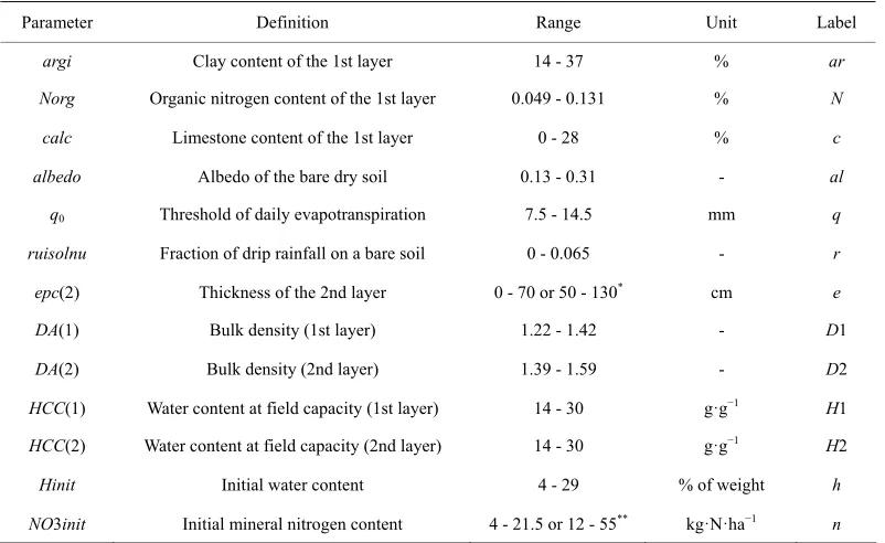
Table 1. Definition of the 13 soil parameters and their ranges of variation.
Parameter Definition Range Unit Label
argi Clay content of the 1st layer 14 - 37 % ar
Norg Organic nitrogen content of the 1st layer 0.049 - 0.131 % N
calc Limestone content of the 1st layer 0 - 28 % c
albedo Albedo of the bare dry soil 0.13 - 0.31 - al
q0 Threshold of daily evapotranspiration 7.5 - 14.5 mm q
ruisolnu Fraction of drip rainfall on a bare soil 0 - 0.065 - r
epc(2) Thickness of the 2nd layer 0 - 70 or 50 - 130* cm e
DA(1) Bulk density (1st layer) 1.22 - 1.42 - D1
DA(2) Bulk density (2nd layer) 1.39 - 1.59 - D2
HCC(1) Water content at field capacity (1st layer) 14 - 30 g·g−1 H1
HCC(2) Water content at field capacity (2nd layer) 14 - 30 g·g−1 H2
Hinit Initial water content 4 - 29 % of weight h
NO3init Initial mineral nitrogen content 4 - 21.5 or 12 - 55** kg·N·ha−1 n
*The first range determine a shallow soil and the second determine a deep soil; **The first range concern the wheat (cultivated after
beet) and the second concern the beet (cultivated after a bare soil).
involved mainly in organic matter decomposition proc- esses. Water content at field capacity of both layers af- fects the water (and nitrogen) movements and storage in the soil reservoir and the thickness of the second layer defines the volume of the reservoir. The initial conditions correspond to the water and nitrogen content, Hinit and
NO3init, at the beginning of the simulation, in this case the sowing date.
2.3. Model Output
In this study, the STICS output variables of interest are:
1) The amount of nitrogen absorbed by the plant (QN) and the leaf area index (LAI) at two (for sugar beet) or three (for wheat) different key stages during the season, which are important variables for making a diagnosis on crop growth,
2) The yield, and the mineral nitrogen content in the soil at harvest (for both crops) plus the grain protein content (for wheat), which are of particular interest for decision making, especially for monitoring nitrogen fer- tilization.
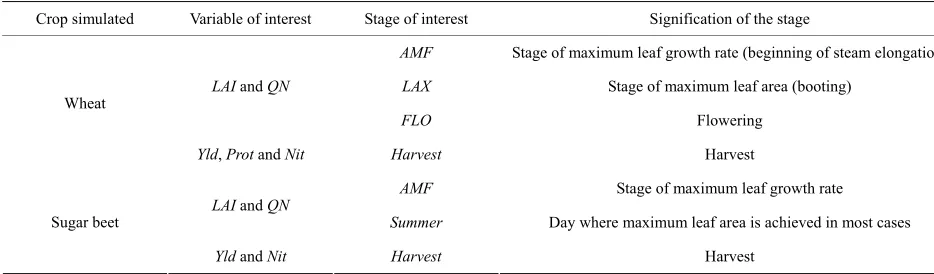
The different stages of interest and the corresponding variables are displayed for each crop on Table 2. For the
wheat, the three key stages concern the maximum leaf growth rate-beginning of stream elongation-(AMF), the maximum leaf area- or booting-(LAX) and the flowering (FLO). For the sugar beet, the two key stages concern the maximum leaf growth rate (AMF) and the maximum leaf
area (Summer).
2.4. Sensitivity and Uncertainty Analysis
Among the available methods of sensitivity analysis, variance-based methods are well adapted for non-linear models that need less than 1 minute for a simulation [36]. These methods are widely used in different contexts [27,28,30-32]. Their principle is to evaluate the contribu- tion of the given uncertain factors to the variance of the model output variables selected. We will describe in this section the sensitivity indices that can be computed with these methods and the EFAST variance-based method we have used in this study to compute these indices. Uncer- tainty analysis is performed here by computing the coef- ficient of variation of the output variables considered from the simulations realized for the sensitivity analysis.
2.4.1. Sensitivity Indices and Coefficient of Variation
We note further Y an output variable of STICS. Y will represent in turn LAI and QN computed at the different phenological stages and the variables computed at har- vest. The total variance of Y, V(Y), is partitioned as fol- lows [37]:
13 1,2, ,131 i 1 13 ij
i i j
V Y V V V
(1)where V(Y) is the total variance of the output variable Y
Table 2. Definition of the variables and the stages of interest.
Crop simulated Variable of interest Stage of interest Signification of the stage
AMF Stage of maximum leaf growth rate (beginning of steam elongation)
LAX Stage of maximum leaf area (booting)
LAI and QN
FLO Flowering
Wheat
Yld, Prot and Nit Harvest Harvest
AMF Stage of maximum leaf growth rate
LAI and QN
Summer Day where maximum leaf area is achieved in most cases Sugar beet
Yld and Nit Harvest Harvest
measures the main effect of the parameter i, i = 1, ···,
13, and the other terms measure the interaction effects. Decomposition (1) is used to derive two types of sensi- tivity indices defined by:
i iV S
V Y
(2)
i iV Y V
ST
V Y
(3)
where V−i is the sum of all the variance terms that do not
include the index i.
Si is the first-order sensitivity index of the ith parame-
ter. It computes the fraction of Y variance explained by the uncertainty of parameter i and represents the main
effect of this parameter on the output variable Y. STi is
the total sensitivity index of the ith parameter and is the sum of all effects (first and higher order) involving the parameter i. Si and STi are both in the range (0, 1), low
values indicating negligible effects, and values close to 1 huge effects. STi takes into account both Si and the inter-
actions between the ith parameter and the 12 other pa- rameters, interactions which can therefore be assessed by the difference between STi and Si. The interaction terms
of a set of parameters represent the fraction of V(Y) in- duced by these parameters but that is not explained by the sum of their main effects. The two sensitivity indices
Si and STi are equal if the effect of the ith parameter on
the model output is independent of the values of the other parameters: in this case, there is no interaction be- tween this parameter and the others and the model is said to be additive with respect to i. Selecting the parameters
that have a negligible effect and that can thus be fixed to nominal values is called factor fixing in the literature [38]. Total effects must be considered in this case. Indeed, a factor that has a small main effect but a medium to high total effect cannot be considered as negligible: its effect depends on the value of other uncertain factors and can be important in some cases.
The coefficient of variation of the output variable Y
can be calculated by:
V Y
YCV Y
Y Y
(4)
where, (Y) is the standard deviation of the output vari- able Y and Y is the mean of Y induced by the 13 soil parameters .
2.4.2. Extended FAST
Sobol’s method and Fourier Amplitude Sensitivity Test (FAST) are two of the most widely used methods to compute Si and STi [11]. We have chosen here to use the
extended FAST (EFAST) method, which has been proved, in several studies [30,39,40], to be more efficient in terms of number of model evaluations than Sobol’s method. The main difficulty in evaluating the first-order and total sensitivity indices is that they require the com- putation of high dimensional integrals. The EFAST algo- rithm performs a judicious deterministic sampling to explore the parameter space which makes it possible to reduce these integrals to one-dimensional ones using Fourier decompositions. The reader interested in a de- tailed description of EFAST can refer to [40].
We have implemented the EFAST method in the Mat- lab® software, as well as a specific tool for computing
and easily handling numerous STICS simulations. The uncertainties considered for the soil parameters are de- scribed in the next section. A preliminary study of the convergence of the sensitivity indices allowed us to set the number of simulations per parameter to 5000, leading to a total number of model runs of 13 × 5000 = 65,000 to compute the main and total effects for all output vari- ables and parameters considered here. One run of the STICS model takes about 1s with a Pentium 4, 2.9 GHz processor.
2.5. Data
ence of sensitivities of different crops to the soil proper- ties. For the same reason, each crop is simulated for two different weathers and two different types of soil depth. The weather data were obtained from the meteorological station of Roupy (49.48˚N, 3.11˚E). The first set of data is chosen to characterize a dry weather (1975-1976) and the second set is chosen to characterize a wet weather (1990-1991). Table 3 shows the amount of rainfall cal-
culated for each season and weather data set. The wheat crop simulated in this study is sown on October 30th while the sugar beet crop is sown on March 30th. The amount of fertilizer provided on wheat varies between 200 kg (shallow soil) and 240 kg (deep soil), while the amount provided on sugar beet varies between 150 kg (shallow soil) and 200 kg (deep soil).
The range of parameter values considered in this study correspond to the soil description of the precision agri- culture experimental site in northern France near Laon, Picardie (Chambry 49.35˚N, 3.37˚E) [41]. In this study, the uncertainties of these 13 soil parameters are observed in the literature (for parameters related to albedo, eva- potranspiration or drip rainfall) or measured in the ex-perimental site (for the other parameters), and their ranges of variation are displayed on Table 1. Concerning
the parameter NO3init two ranges of variation are con- sidered, depending on the crop cultivated just before the one considered: in this study, the wheat is cultivated after sugar beet and the sugar beet is cultivated after a bare soil. The different previous crops used determine the quantity of nitrogen NO3init at the beginning of the cor- responding crop season. The two different types of soil depth are defined by their ranges of variation (Table 1)
and correspond to a shallow soil and a deep soil. The uncertainties considered in the global sensitivity analysis for the soil parameters are assumed independent and fol- low uniform distributions. The ranges of variation of the distributions are given in Table 1.
3. RESULTS AND DISCUSSION
Only the main results of the study are presented here for the sake of clarity. These results concern: 1) wheat crop simulated with dry, then wet weather and a shallow soil and 2) sugar beet crop simulated with dry, then wet weather and a deep soil.
3.1. Global Sensitivity Analysis
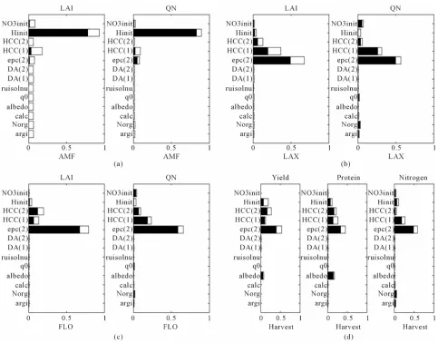
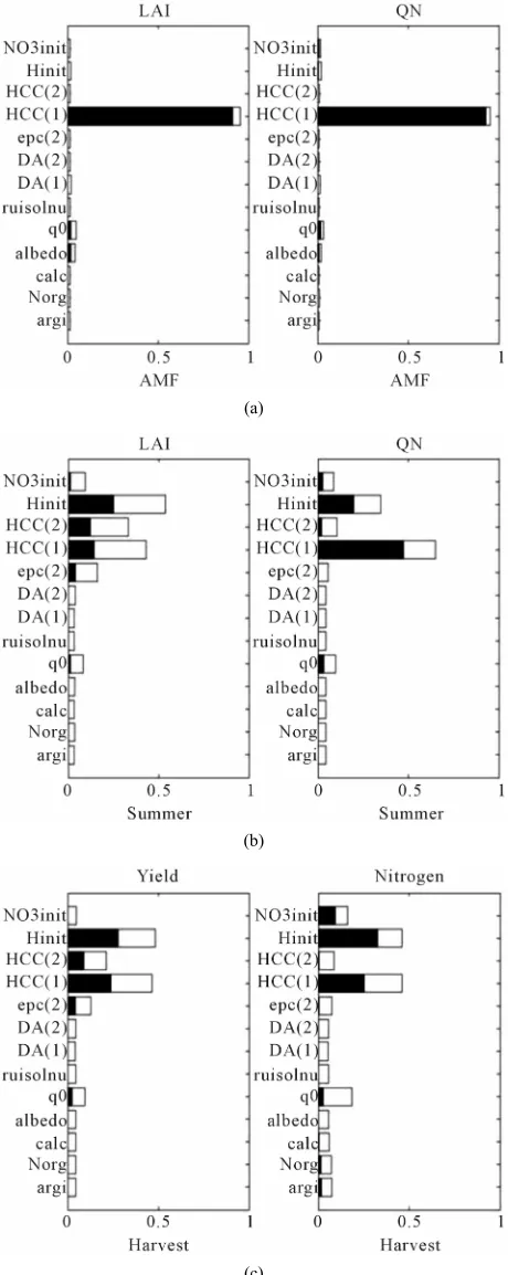
Figure 1 shows the sensitivity indices calculated for
the 13 soil parameters and for each output variable of the wheat crop simulated with a dry weather and a shallow soil. For the early stage the initial water content is domi- nant because in the considered weather, the rainfall is light in autumn when the wheat is sown (see Table 3): at
the stage AMF (Figure 1(a)), Hinit is the only parameter
Table 3. Amount of rainfall (in mm) calculated for each season and weather.
Spring Summer Autumn Winter Dry weather 343.4 167.8 222.4 218.8
Wet weather 361.4 247.9 239.4 316.4
contributing (for more than 90%) to the output variance for both variables LAI and QN. In the later stages, the effects of parameters evolve with the soil volume ex- plored by the roots (first layer, then second one), up to the flowering stage where the root development is maximum: at the stage LAX (Figure 1(b)) and FLO
(Figure 1(c)), the effect of Hinit disappears and that of HCC(1) and epc(2) increase, with a dominant position of
epc(2). At Harvest (Figure 1(d)), the variables are much
sensitive to epc(2) followed by HCC(1), HCC(2) and
Hinit for the three variables and albedo for the variable protein of the grain. In those conditions of dry weather and shallow soil, the parameters related to water avail- ability (epc(2), HCC(1), HCC(2) and Hinit) are the main parameters contributing to the variance of the outputs. Those concerned by the turnover of organic nitrogen in the soil are not concerned, because the water stress is the dominant limiting factor and also because the minerali- zation processes are reduced by dry conditions.
When considering wet conditions (Figure 2), the wa-
ter stress is not so much a limiting factor: maximum LAI
is equal to 3.61 in average, whereas it is equal to 2.57 in dry conditions (see Table 4). The roots grow more rap-
idly at the beginning of the season and the size of the soil reservoir (via the parameter epc(2)) is important since the AMF stage: the depth of roots is equal to 55.84 in average (3 months after the sowing), whereas it is equal to 45.62 in dry conditions (see Table 4). Moreover, in
these conditions, the mineralization of the soil organic matter is increased and the effects of the concerned pa- rameters argi and Norg do so: the cumulative mineral nitrogen arising from humus is equal to 23.95 in average (at stage LAX), whereas it is equal to 18.09 in dry condi- tions (see Table 4). This does not seem to influence the
effects of the different parameters on LAI at stage AMF
since they are very similar to these obtained with the dry weather. On the contrary, the sensitivities of the variable
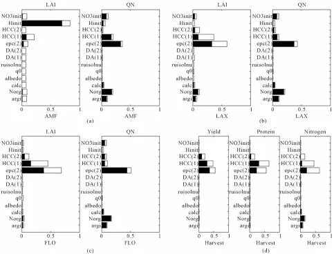
QN to the different parameters are very different from the ones obtained with a dry weather: there is no contribu- tion of Hinit but epc(2), HCC(1) and parameters in- volved in the mineralization process (argi, Norg and
NO3init) contribute to the output variance.
This is also the case for both LAI and QN on later stages, with an increasing dominancy of epc(2). At Har- vest (Figure 2(d)), the variables are sensitive to the pa-
Figure 1. Sensitivity indices of the 13 soil parameters for each model output of the wheat crop simulated with a dry weather and a shallow soil. The outputs (a) correspond to LAI and QN at stage AMF; (b) correspond to LAI and QN at stage LAX; (c) correspond to
LAI and QN at stage FLO and (d) correspond to Yld, Prot and Nit at Harvest. First-order indices are in black and interactions in white.
content. The main difference between these results and those presented in Figure 1 lies in the sensitivity to pa-
rameters involved in the mineralization process (espe- cially argi and Norg).
When considering wet conditions (Figure 2), the wa-
ter stress is not so much a limiting factor: maximum LAI
is equal to 3.61 in average, whereas it is equal to 2.57 in dry conditions (see Table 4). The roots grow more rap-
idly at the beginning of the season and the size of the soil reservoir (via the parameter epc(2)) is important since the AMF stage: the depth of roots is equal to 55.84 in average (3 months after the sowing), whereas it is equal to 45.62 in dry conditions (see Table 4). Moreover, in
these conditions, the mineralization of the soil organic matter is increased and the effects of the concerned pa- rameters argi and Norg do so: the cumulative mineral nitrogen arising from humus is equal to 23.95 in average (at stage LAX), whereas it is equal to 18.09 in dry condi-
tions (see Table 4). This does not seem to influence the
effects of the different parameters on LAI at stage AMF
since they are very similar to these obtained with the dry weather. On the contrary, the sensitivities of the variable
QN to the different parameters are very different from the ones obtained with a dry weather: there is no contribu- tion of Hinit but epc(2), HCC(1) and parameters in- volved in the mineralization process (argi, Norg and
NO3init) significantly contributes to the variance of this variable. This is also the case for both LAI and QN on later stages, with an increasing dominancy of epc(2). At
Harvest (Figure 2(d)), the variables are sensitive to the
parameters epc(2), HCC(1) and HCC(2) with still a slight sensitivity to argi and Norg for the soil mineral nitrogen content. The main difference between these results and those presented in Figure 1 lies in the sensitivity to pa-
Figure 2. Sensitivity indices of the 13 soil parameters for each model output of the wheat crop simulated with a wet weather and a shallow soil. The outputs (a) correspond to LAI and QN at stage AMF; (b) correspond to LAI and QN at stage LAX; (c) correspond to
[image:7.595.59.537.550.652.2]LAI and QN at stage FLO and (d) correspond to Yld, Prot and Nit at Harvest. First-order indices are in black and interactions in white.
Table 4. Ranges of some output variables uncertainties generated by the uncertainties on the soil parameters. The output concerns the value of maximum LAI, the cumulative mineral nitrogen arising from humus Qminh (calculated at the stage LAX or Summer) and the depth of roots Zrac (calculated 3 months after the sowing date).
Maximum LAI Qminh Zrac
Configuration of simulation*
min mean max min mean max min mean max
W C1– 0.78 2.57 3.73 7.19 18.09 40.51 30.1 45.62 56.52
W C2– 2.51 3.61 5.08 9.8 23.95 48.85 30.1 55.84 69.91
SB C1+ 0 1.42 4.61 0 24.91 83.38 12.06 77.58 129.61
SB C2+ 0.19 4 6.06 19.19 50.19 121.45 71.08 85.55 102.58
*Wheat crop, shallow soil and dry weather (W C1–) or wet weather (W C2–); sugar beet crop, deep soil and dry weather (SB C1 +) or wet weather (SB C2 +).
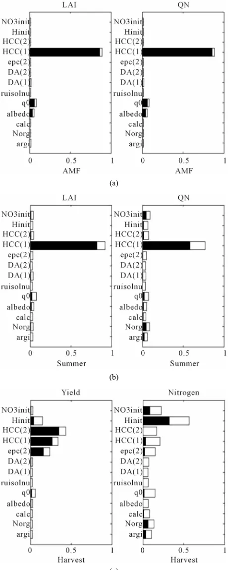
Figure 3 shows the sensitivity indices calculated for
the 13 soil parameters and for each output variable of the sugar beet crop simulated with a deep soil and a dry weather. In this case, the crop grows mainly in summer where it experiences a severe water stress, leading to a
value of maximum LAI equal to 1.42 in average (see Ta- ble 4). The depth of the second layer (parameter epc(2))
(a)
(b)
[image:8.595.57.287.86.663.2](c)
Figure 3. Sensitivity indices of the 13 soil parameters for each model output of the sugar beet crop simulated with a dry weather and a deep soil. The outputs (a) correspond to LAI and
QN at stage AMF; (b) correspond to LAI and QN at Summer
and (c) correspond to Yld and Nit at Harvest. First-order indices are in black and interactions in white.
thickness of soil (the depth of roots is equal to 77.58 in average), the output variables are no longer sensitive to the parameter epc(2) when the soil is deep. Moreover, the outputs are not at all sensitive to the initial water content
Hinit because the amount of rainfall is quite important in spring, when the sugar beet is sown (see Table 3). The
soil water reserve is therefore the main limiting factor and it depends only on HCC(1) for the early stage AMF: it contributes for 95% of the total output variance of LAI
and QN. For the Summer stage (Figure 3(b)), which cor-
respond to the maximum of water stress index, LAI is mainly sensitive to parameters linked to water availabil- ity of both soil layers (HCC(1) and HCC(2)) with an increase of the sensitivity to Hinit. QN is more sensitive to characteristics of the top layer (HCC(1) and Hinit) where is concentrated the organic nitrogen, as it influ- ences the fate of available nitrogen coming from miner- alization. The same tendencies are noticed for the output variables at Harvest, the yield being more linked to LAI
and soil mineral nitrogen to QN. Many interactions are visible between all these parameters. It is also noticeable that, as in the case of wheat, the output variables have very low sensitivity to the parameters concerned with nitrogen turnover in the soil, due to the dry weather and limited mineralization. The main differences of these results with respect to those presented for the wheat crop (Figures 1 and 2) is: 1) that HCC(1) contributes a lot to
the variance of the output variables during all the crop season; 2) that Hinit has no contribution to the variance of the output variables at the beginning of the sugar beet season and 3) that epc(2) does not affect the output vari- ables when the soil is deep.
When considering wet conditions (Figure 4), the sugar
beet crop growth is less affected by the water stress: maximum LAI is equal to 4 in average, whereas is equal to 1.42 in dry conditions (see Table 4). The soil water
reserve of the second layer is not a limiting factor in deep soil and wet conditions for both stages AMF and Summer
because the soil reservoir has a large size and the water stress is low. Thus, LAI and QN are only sensitive to the soil water reserve of the first layer which only depends on HCC(1) (it does not depend on Hinit because of the high amount of rainfall in spring). Nevertheless, the soil water reserve of the second layer becomes a limiting factor at the end of the sugar beet crop season, when the roots are deep, involving a significant sensitivity of the output Yld to the parameters HCC(1), HCC(2) and epc(2). Moreover, the mineralization of the soil organic matter slightly increases in wet conditions and so do the effects of the concerned parameters on QN at Summer and Nit at yield: the cumulative mineral nitrogen arising from hu- mus is equal to 50.19 in average, whereas is equal to 24.91 in dry conditions (see Table 4). The main difference be-
(a)
(b)
(c)
Figure 4. Sensitivity indices of the 13 soil parameters for each model output of the sugar beet crop simulated with a wet weather and a deep soil. The outputs (a) correspond to LAI and
QN at stage AMF; (b) correspond to LAI and QN at Summer
and (c) correspond to Yld and Nit at Harvest. First-order indices are in black and interactions in white.
in the lower sensitivity of the soil water reserve parame- ters of the second layer at the two first stages of interest.
3.2. Total Effect and Coefficient of Variation
[image:9.595.57.287.86.661.2]For each configuration of simulation presented above,
Figure 5 shows the coefficient of variation CV of each
output variable and the corresponding total effect ST of each parameter. The horizontal dashed line is situated at an arbitrary minimum value ST = 10% and the vertical dashed line is situated at another arbitrary minimum value CV = 1/3. The threshold of 10% for ST has been proposed by [30] for screening the significant sensitivity values. When wheat crop is simulated with a dry weather and a shallow soil (see Figure 5(a)), three output vari-
ables have a coefficient of variation higher than 1/3: Prot
(CV = 0.37), Yld (CV = 0.54) and LAI at the stage FLO
(CV = 0.62). For these outputs, only 5 soil parameters have a ST higher than 10%: epc(2), HCC(1), HCC(2),
Hinit and albedo. This means that for simulating cor-
rectly these output variables of the wheat crop when the weather is dry and the soil depth is shallow, only epc(2),
HCC(1), HCC(2), Hinit and albedo have to be deter- mined accurately and the other parameters can be fixed at a nominal value (assuming the arbitrary thresholds ST
= 10% and CV = 1/3). When wheat crop is simulated with a wet weather and a shallow soil (Figure 5(b)), only
the variable Nit has a coefficient of variation slightly higher than 1/3 (CV = 0.38). The corresponding parame- ters having a ST higher than 10% are epc(2), HCC(1),
HCC(2) and Norg, meaning that these parameters are important to be determined accurately for simulating correctly the wheat crop in this case. The first main dif-ference between the results presented in Figures 5(a) and (b) is that only one output variable has a CV higher than
1/3 when the weather is wet, instead of three when the weather is dry. The second main difference is that the parameters albedo and Hinit, which contribute for a sig- nificant part of the output variance when the weather is dry, are replaced by the parameter Norg, which is in- volved in the mineralization process and contribute for a significant part of the variance of the outputs when the weather is wet.
Considering the results presented in Figures 5(a) and (b), the parameter Hinit, which contributes for a large
Figure 5. Coefficient of variation CV of each output variables and the corresponding total effects ST of the 13 soil parameters. The horizontal dashed line is situated at ST = 10% and the vertical dashed line is situated at CV = 1/3. The outputs are simulated for (a) wheat crop, dry weather and shallow soil, (b) wheat crop, wet weather and shallow soil, (c) sugar beet crop, dry weather and deep soil and (d) sugar beet crop, wet weather and deep soil. Label C1 correspond to the dry weather and C2 to the wet one, W correspond to the wheat crop and SB to sugar beet, − correspond to a shallow soil and + to a deep one. Parameter labels are presented in Table 1.
thought. The parameter epc(2), which contributes for a large part to the variance of all the output variables dur- ing all the wheat crop season (see Section 3.1), proves to be the most important parameter to be determined accu- rately for simulating the wheat crop when the type of soil depth is shallow.
The Figure 5(c) shows the results when the sugar beet
crop is simulated with a dry weather and a deep soil. It reveals that all the output variables have a coefficient of variation higher than 1/3 meaning that the uncertainties on the soil parameters generate a large uncertainty on the considered variables. Among those parameters, five need to be measured accurately: epc(2), HCC(1), HCC(2),
Hinit and q0. The main difference between the results
presented in Figures 5(a) and (c) is that all the output
variables are strongly affected by the measurement of the soil parameters when the sugar beet is simulated. When sugar beet is simulated with a deep soil and a wet weather (Figure 5(d)), only the output variables LAI and
QN at the stage AMF and Nit have a CV higher than 1/3 (resp. CV = 0.54, 0.53 and 0.68). For LAI and QN at the stage AMF, the only parameter having a ST higher than 10% is HCC(1). For Nit, a lot of parameters exceeds this threshold: argi, Norg, q0, epc(2), HCC(1), HCC(2), Hinit
and NO3init. It is thus necessary to determine accurately a lot of parameters for simulating correctly the output Nit, while it is necessary to determine only one parameter for simulating correctly LAI and QN at AMF.
When sugar beet is simulated with a deep soil and a wet weather (Figure 5(d)), only the output variables LAI
and QN at the stage AMF and Nit have a CV higher than 1/3 (resp. CV = 0.54, 0.53 and 0.68). For LAI and QN at the stage AMF, the only parameter having a ST higher than 10% is HCC(1). For Nit, a lot of parameters exceeds this threshold: argi, Norg, q0, epc(2), HCC(1), HCC(2),
parameter for simulating correctly LAI and QN at AMF. The main difference between these results and those presented in Figure 5(c) is that, excepted for the output Nit, at most one parameter has to be accurately known for simulating correctly the sugar beet crop in deep soil and wet conditions. The parameter HCC(1), which con- tributes for a large part to the variance of all the output variables during all the sugar beet crop season (see Sec- tion 3.1), proves to be the most important parameter to be measured accurately for simulating the sugar beet crop when the soil is deep.
4. CONCLUSIONS
Global sensitivity analysis is an interesting tool for ranking parameters with respect to their contribution to the variance of the output variables of a model. However, the only use of sensitivity indices proves to be unsatis- factory for deciding which parameters should be accu- rately measured in a given configuration. Only the com- bination of uncertainty and sensitivity analysis is relevant to reach this goal. We propose in this study a simple and easy to use method that combines these two analysis in order to select the parameters that needs particular accu- racy for simulating a set of variables of interest with an acceptable precision. This method, which can be easily applied to any crop model and group of parameters, has three steps: 1) compute the global sensitivity indices for each uncertain parameter; 2) compute the coefficient of variation of the outputs of interest from the set of simula- tions performed at step 1); and 3) select the parameters to be accurately measured for simulating correctly these outputs by setting thresholds on sensitivity indices and coefficients of variation. Of course the results of this method are strongly linked to the uncertainties hypothe- sized for the parameters and special attention must be paid to this aspect. Coefficients of variation and sensitiv- ity indices thresholds should be adapted to each case depending on the level of measurements constraints and of the accuracy wishes for model output simulations.
We apply this method to the crop model STICS for selecting soil parameters that need to be measured at a field scale. Practically this needs the knowledge of the conditions under which the crop grows (weather, type of soil depth, agricultural techniques…) and it has been shown here that the results depend on these conditions. Moreover, the field scale variability of soil parameters, assumed in this application, gives a larger importance to parameters related to water availability than those related to mineralization. Concerning non-permanent soil pa- rameters such as initial conditions, the application of the method needs thus to be based on future scenarios. This application shows that the number of STICS soil pa- rameters to be measured accurately for simulating cor-
rectly the output variables considered here for wheat and sugar beet crops (given the parameters uncertainties used and in the configurations studied) can be significantly reduced by the use of this method. This is of particular interest given the time and financial cost of soil meas- urements.
REFERENCES
[1] Batchelor, W.D., Basso, B. and Paz, J.O. (2002) Exam- ples of strategies to analyze spatial and temporal yield variability using crop models. European Journal of Agro- nomy, 18, 141-158. doi:10.1016/S1161-0301(02)00101-6 [2] Gabrielle, B., Roche, R., Angas, P., Cantero-Martinez, C.,
Cosentino, L., Mantineo, M., Langensiepen, M., Henault, C., Laville, P., Nicoullaud, B. and Gosse, G. (2002) A pri-ori parameterisation of the CERES soil-crop models and tests against several European data sets. Agronomie, 22, 119-132. doi:10.1051/agro:2002003
[3] Houlès, V., Mary, B., Guérif, M., Makowski, D. and Juste, E. (2004) Evaluation of the crop model STICS to recom- mend nitrogen fertilization rates according to agro-envi- ronmental criteria. Agronomie, 24, 1-9.
doi:10.1051/agro:2004036
[4] Launay, M. and Guérif, M. (2003) Ability for a model to predict crop production variability at the regional scale: An evaluation for sugar beet. Agronomie, 23, 135-146.
doi:10.1051/agro:2002078
[5] Tremblay, M. and Wallach, D. (2004) Comparison of parameter estimation methods for crop models. Agronomie, 24, 351-365. doi:10.1051/agro:2004033
[6] Varella, H., Guérif, M., Buis, S. and Beaudoin, N. (2010) Soil properties estimation by inversion of a crop model and observations on crop improves the prediction of agro- environmental variables. European Journal of Agronomy, 33, 139-147. doi:10.1016/j.eja.2010.04.005
[7] Flenet, F., Villon, P. and Ruget, F.O. (2003) Methodology of adaptation of the STICS model to a new crop: Spring linseed (Linum usitatissimum, L.). STICS Workshop, Camargue, FRANCE, 367-381.
[8] Hadria, R., Khabba, S., Lahrouni, A., Duchemin, B., Chehbouni, A., Carriou, J. and Ouzine, L. (2007) Calibra-tion and validaCalibra-tion of the STICS crop model for manag-ing wheat irrigation in the semi-arid Marrakech/Al Haouzi plain. Arabian Journal for Science and Engi-neering, 32, 87-101.
[9] Singh, A.K., Tripathy, R. and Chopra, U.K. (2008) Eva- luation of CERES-Wheat and CropSyst models for water- nitrogen interactions in wheat crop. Agricultural Water Management, 95, 776-786.
doi:10.1016/j.agwat.2008.02.006
[10] Guérif, M. and Duke, C. (1998) Calibration of the SU-CROS emergence and early growth module for sugar beet using optical remote sensing data assimilation. European Journal of Agronomy, 9, 127-136.
doi:10.1016/S1161-0301(98)00031-8
Parameterizing spatial crop models with inverse modeling: Sources of error and unexpected results. Transactions of the Asabe, 49, 1547-1561.
[12] Irmak, A., Jones, J.W., Batchelor, W.D. and Paz, J.O. (2001) Estimating spatially variable soil properties for application of crop models in precision farming. Transac- tions of the ASAE, 44, 1343-1353.
[13] Nemes, A., Timlin, D.J., Pachepsky, Y.A. and Rawls, W.J. (2009) Evaluation of the Rawls et al. (1982) Pedotransfer Functions for their Applicability at the US National Scale.
Soil Science Society of America Journal, 73, 1638-1645. [14] King, D., Daroussin, J. and Tavernier, R. (1994)
Devel-opment of a soil geographic database from the soil map of the European communities. Catena, 21, 37-56.
doi:10.1016/0341-8162(94)90030-2
[15] Bourennane, H., King, D., Couturier, A., Nicoullaud, B., Mary, B. and Richard, G. (2007) Uncertainty assessment of soil water content spatial patterns using geostatistical simulations: An empirical comparison of a simulation accounting for single attribute and a simulation account-ing for secondary information. Ecological Modelling, 205, 323-335. doi:10.1016/j.ecolmodel.2007.02.034
[16] Samouelian, A., Cousin, I., Tabbagh, A., Bruand, A. and Richard, G. (2005) Electrical resistivity survey in soil science: A review. Soil & Tillage Research, 83, 173-193.
doi:10.1016/j.still.2004.10.004
[17] Braga, R.P. and Jones, J.W. (2004) Using optimization to estimate soil inputs of crop models for use in site-specific management. Transactions of the ASAE, 47, 1821-1831. [18] Varella, H., Guérif, M. and Buis, S. (2010) Global
sensi-tivity analysis measures the quality of parameter estima-tion: The case of soil parameters and a crop model. Envi-ronmental Modelling & Software, 25, 310-319.
doi:10.1016/j.envsoft.2009.09.012
[19] Bouman, B.A.M. (1994) A framework to deal with un-certainty in soil and management parameters in crop yield simulation: A case-study for rice. Agricultural Systems, 46, 1-17. doi:10.1016/0308-521X(94)90166-D
[20] St'astna, M. and Zalud, Z. (1999) Sensitivity analysis of soil hydrologic parameters for two crop growth simula-tion models. Soil & Tillage Research, 50, 305-318.
doi:10.1016/S0167-1987(99)00021-5
[21] Saltelli, A., Chan, K. and Scott, E.M. (2000) Sensitivity analysis. John Wiley and Sons, New York.
[22] Aggarwal, P.K. (1995) Uncertainties in crop, soil and weather inputs used in growth-models: Implications for simulated outputs and their applications. Agricultural Systems, 48, 361-384.
doi:10.1016/0308-521X(94)00018-M
[23] Blasone, R.S., Madsen, H. and Rosbjerg, D. (2008) Un-certainty assessment of integrated distributed hydrologi-cal models using GLUE with Markov chain Monte Carlo sampling. Journal of Hydrology, 353, 18-32.
doi:10.1016/j.jhydrol.2007.12.026
[24] Lawless, C., Semenov, M.A. and Jamieson, P.D. (2008) Quantifying the effect of uncertainty in soil moisture characteristics on plant growth using a crop simulation model. Field Crops Research, 106, 138-147.
doi:10.1016/j.fcr.2007.11.004
[25] Tolson, B.A. and Shoemaker, C.A. (2008) Efficient pre-diction uncertainty approximation in the calibration of environmental simulation models. Water Resources Re-search, 44, W04411. doi:10.1029/2007WR005869 [26] Van der Keur, P., Hansen, J.R., Hansen, S. and Refsgaard,
J.C. (2008) Uncertainty in simulation of nitrate leaching at field and catchment scale within the odense river basin.
Vadose Zone Journal, 7, 10-21.
doi:10.2136/vzj2006.0186
[27] Campolongo, F. and Saltelli, A. (1997) Sensitivity analy-sis of an environmental model an application of different analysis methods. Reliability Engineering & System Safety, 57, 49-69. doi:10.1016/S0951-8320(97)00021-5
[28] Gomez-Delgado, M. and Tarantola, S. (2006) GLOBAL sensitivity analysis, GIS and multi-criteria evaluation for a sustainable planning of a hazardous waste disposal site in Spain. International Journal of Geographical Informa-tion Science, 20, 449-466.
doi:10.1080/13658810600607709
[29] Lamboni, M., Makowski, D., Lehuger, S., Gabrielle, B. and Monod, H. (2009) Multivariate global sensitivity analysis for dynamic crop models. Field Crops Research, 113, 312-320. doi:10.1016/j.fcr.2009.06.007
[30] Makowski, D., Naud, C., Jeuffroy, M.H., Barbottin, A. and Monod, H. (2006) Global sensitivity analysis for calculating the contribution of genetic parameters to the variance of crop model prediction. Reliability Engineer-ing & System Safety, 91, 1142-1147.
doi:10.1016/j.ress.2005.11.015
[31] Pathak, T.B., Fraisse, C.W., Jones, J.W., Messina, C.D. and Hoogenboom, G. (2007) Use of global sensitivity analysis for CROPGRO cotton model development. Trans- actions of the ASABE, 50, 2295-2302.
[32] Saltelli, A., Tarantola, S. and Campolongo, F. (2000) Sen- sitivity analysis as an ingredient of modeling. Statistical Science, 15, 377-395. doi:10.1214/ss/1009213004
[33] Brisson, N., Launay, M., Mary, B. and Beaudoin, N. (2008) Conceptual basis, formalisations and parameteri-zation of the STICS crop model. Quae, Versailles. [34] Brisson, N., Ruget, F., Gate, P., Lorgeou, J., Nicoullaud,
B., Tayot, X., Plenet, D., Jeuffroy, M.H., Bouthier, A., Ripoche, D., Mary, B. and Juste, E. (2002) STICS: A ge-neric model for simulating crops and their water and ni-trogen balances. II. Model validation for wheat and maize.
Agronomie, 22, 69-92. doi:10.1051/agro:2001005
[35] Launay, M., Graux, A.-I., Brisson, N. and Guérif, M. (2009) Carbohydrate remobilization from storage root to leaves after a stress release in sugar beet (Beta vulgaris
L.): Experimental and modelling approaches. The Journal of Agricultural Science, 147, 669-682.
doi:10.1017/S0021859609990116
[36] Cariboni, J., Gatelli, D., Liska, R. and Saltelli, A. (2004) The role of sensitivity analysis in ecological modelling. 4th Conference of the International Society for Ecological Informatics, Busan, 24-28 October 2004, 167-182. [37] Chan, K., Tarantola, S., Saltelli, A. and Sobol, I.M. (2001)
Scott, E.M., Eds., Sensitivity Analysis, Wiley, New York, 167-197.
[38] Ratto, M., Young, P.C., Romanowicz, R., Pappenberger, F., Saltelli, A. and Pagano, A. (2007) Uncertainty, sensi- tivity analysis and the role of data based mechanistic modeling in hydrology. Hydrology and Earth System Sci- ences, 11, 1249-1266. doi:10.5194/hess-11-1249-2007 [39] Saltelli, A. and Bolado, R. (1998) An alternative way to
compute Fourier amplitude sensitivity test (FAST). Com- putational Statistics & Data Analysis, 26, 445-460.
doi:10.1016/S0167-9473(97)00043-1
[40] Saltelli, A., Tarantola, S. and Chan, K.P.S. (1999) A quan- titative model-independent method for global sensitivity analysis of model output. Technometrics, 41, 39-56.
doi:10.1080/00401706.1999.10485594