Reuse oriented SLAM framework using component based approach

(1)

Reuse-oriented SLAM Framework using

Component-based Approach

M.A. (Mohamed) Abdelhady

MSc Report

C

e

Prof.dr.ir. S. Stramigioli

Dr.ir. D. Dresscher

Dr.ir. J.F. Broenink

Dr. M Poel

August 2017

040RAM2017

Robotics and Mechatronics

EE-Math-CS

University of Twente

(2)

(3)

iii

Summary

Simultaneous Localization and Mapping also known asSLAM is a well established problem in the scientific community and considered to be solved for a specific combination of en-vironment, resources and requirements. It depicts the process of a robot creating a map of an unknown environment while simultaneously estimating its location within the self-created map. Currently, numerous SLAM algorithms have been successfully developed and applied to a multitude of applications using different platforms. The motivation for this work is the lack of a formal development methodology for SLAM and the tight coupling of the constituting sub-modules of the software artifacts, which reflects poorly on code reusability. Henceforth, a reuse-oriented framework is sought that aims at decoupling SLAM and reducing the devel-opment and deployment time. The framework is built usingcomponent-based software devel-opmentapproaches which is utilized to encapsulate the different parts in SLAM as software components and enforce the separation of concerns.

(4)

Preface

This report constitutes as a documentation for my master thesis done at the Robotics & Mecha-tronics group at the University of Twente. The work is done as a part ofi-Boticsproject.

I am thankful for all the learning opportunities I had, and for everyone who supported me along the way.

Kind regards,

Mohamed A. Abdelhady

(5)

v

1 Introduction

1.1 Problem formulation

SLAM refers to the task of simultaneous localization and mapping, which is a well investigated problem in robotics and photogrammetry (also known asStructure from Motion (SfM)). It can be briefly described as a robot attempting to localize itself through an unknown environment and simultaneously create a map of this environment while navigating it. The robot is equipped with multiple information sources which provide the required perception inputs. The main challenge of the problem is the cyclic dependency between both tasks, namely, localization and mapping. i.e. the location is required to create the map and the map is in turn required to determine the location.

SLAM is applied to numerous fields such as warehouse management, port automation, seabed mapping, self-driving cars, commercial indoor robots, space exploration and many more.

Several SLAM algorithms have been successfully used in multiple applications with specific combinations of robot, environment, algorithm and performance. This includes for example indoor mapping of small areas or even buildings using mobile robot and UAVs equipped with laser scanners. Underwater mapping of seabed has also been successful to some extent. How-ever, it is still a challenging task in rough terrains, fast dynamic behavior, large outdoor envi-ronments, etc. Cadena et al. (2016) comprehensively discusses the open challenges in SLAM and the trend towards robustness in robot perception.

As a final product, SLAM is a relatively complex software artifact. It is often developed to show-case the feasibility of a novel algorithm or to improve upon existing approaches. The result is a source code that is relatively inflexible and requires extensive efforts to be reused. Remark-ably few contributions have addressed the issue of reusability and attempted to create a formal design methodology of SLAM as a software, although SLAM was firstly developed in the 1980s and witnessed many development cycles [Durrant-Whyte and Bailey (2006)].

The reuse of SLAM is becoming a pressing matter as it has been expanding towards applications in mature domains such as automotive industries. Hence, it has to comply with the industrial standards already present in these domains. These standards include non-functional specifi-cations that relates to the maturity of the software such as reliability, reusability, security, etc.

1.2 Approach

Therefore, from the point of view of the different stakeholders it is advantageous to introduce unification and standardization to the design and development processes by creating an in-frastructure which can be extended to accommodate all the variabilities of SLAM. Hence, a reuse-oriented framework is sought that adopts component-based software approaches in or-der to improve the quality of the software products and reduce the time of deployment, it can also provide a flexible way of handling addition or adjustments to algorithms and plat-forms(sensors, robots, middleware, etc.).

Through following this development strategy the different SLAM modules will be decoupled allowing easier maintenance, debugging, extension and replacement. Accordingly, these tasks can be done in a complete standalone fashion without the need to modify or write extra glue code for the already existing ones. This is in contrast to the approach of having a single code block or a monolithic architecture which performs all the different functionalities.

The main research objective is to:

(8)

1.3 Related work

The field of robotics can greatly make use of the tools and techniques developed in software engineering in order to analyze, test and design complex systems. It is essential to exploit the synergy between both domains.

Several projects have already been exploring the overlapping areas between both fields, a sum-mary of which is given as follows: Brugali et al. (2012) applies software product line approach to refactor navigation libraries available in the ROS environment and the resulting architecture is shown to be more modular and middleware independent, Bruyninckx et al. (2013) presents a seminal work demonstrating best practices in developing software components from robotics by promoting the separation of concerns and model-driven engineering, Ristroph (2008) at-tempts at developing early steps for modular SLAM, Foxlin (2002) illustrates a general archi-tecture for localization, auto-calibration and mapping by using a decentralized Kalman filter, Ratasich et al. (2015) demonstrates a generic sensor fusion package for ROSsf-pkgthat is able to handle the combination of an arbitrary number of any single-dimension value sensor, Moore T. ; Stouch (2014) also develops a modulars sensor fusion package for ROS based on an extended Kalman filterethz_msf, Blumenthal et al. (2011) surveys and applies refactoring techniques to commonly used robotic perception libraries yielding a reusable set of software components with harmonized interfaces, and Ball et al. (2013) presentsOpenRatSLAMa ROS open-source version of RatSLAM in a middleware independent fashion with software architecture docu-mentation of the different components.

1.4 Outline

(9)

3

2 Background

This chapter provides the reader with the background material regarding SLAM and the paradigms of component-based software development and software product lines.

2.1 A brief introduction into SLAM

SLAM is the process describing the navigation of a mobile robot in an unknown environment in order to create a map of the surroundings while simultaneously inferring its own location within the self-created map. This is considered to be one of the most important functionalities a mobile robot must posses in order to become truly autonomous [Siciliano and Khatib (2016)]. In order to introduce the basic concepts and notations, the classical probabilistic framework will be used. It should be noted that this specific SLAM representation is not exclusive and the general problem can be expressed using many different formulations [Strasdat et al. (2010)].

Theposeof the robot which is to be estimated at a certain time instance is represented by the state variablext, where the dimension ofxt is context dependent. For the simple case of a

planar mobile robotxt∈R3as it consists of the 2D coordinates and the headingxt=(x,y,θ)T.

The map of the environmentm is the second variable to be estimated. It can take different forms depending on the chosen map representation which can be feature-based, volumetric or topological. It is often assumed that the map is static and therefore does not evolve with time.

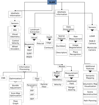
The information that is provided to the robot can be classified into two classes; theidiothetic1

information which is related to the self-motion cues and is regarded as control inputut. This

information can be retrieved from velocity commands, wheel encoders, inertial measurement units, etc. The second class of information that is utilized is theallothetic2information which is related to the external cues. This could be represented as a distinct landmark in the environ-ment that the robot can observe and deduce its relative pose. The measureenviron-ments are denoted aszt.

The robot then seeks to calculate the conditional probability function presented in Eq. 2.1 [Thrun et al. (2005)], which estimates the robot’s posextand the mapmbased on the idiothetic

and allothetic information given asut andzt respectively. It is important to emphasize that in

certain SLAM approaches, the term representing the mapmis often incorporated within the state vectorxt.

p(xt,m|z1:t,u1:t) (2.1)

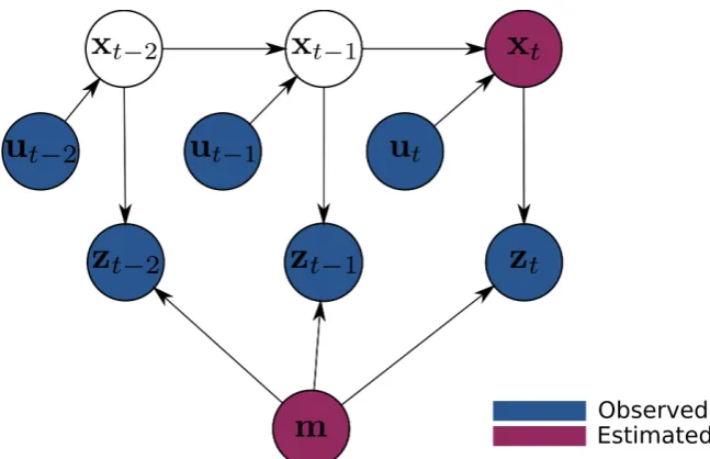
The graphical model shown in Fig. 2.1 shows the four main variables involved in SLAM. It also highlights the desired map and pose estimates. One can also distinguish between the values which are directly observed by the robot and which are estimated. Finally, the arrows indicate a causal relationship, for example, the pose of the robot at timet is influenced by the pose at timet1and the control inputut.

2.1.1 Taxonomy

A great number of SLAM variants have been developed; they can be categorized along different dimensions that as explained extensively in Thrun et al. (2005) and Siciliano and Khatib (2016), the commonly used classifications are given as follows:

(10)

[image:10.595.122.446.75.284.2]

Figure 2.1:Graphical model of the online SLAM problem. The robot is provided with control inputut

and measurementszt, and it is required to estimate its own posextand the map of the environmentm

[Thrun et al. (2005)].

• Online versus offline, where online approach tries to estimate only the current pose of the robot and disregards the past poses, in contrast with the offline approach which tries to find the optimal path of the robot consisting of all previous poses. Both variants are of equal importance in practice.

• Active versus passive, where in active SLAM the direction of the robot motion is con-trolled purposefully to produce an more accurate estimate. On the other hand, the pas-sive approach does not interfere with the control of the robot and allows for free roaming.

• Static versus dynamic, where the environment is assumed to either change over time and the dynamic effects can be detected or as static where it does not change.

Several strategies has been developed in order to solve the conditional probability described by Eq. 2.1 and will later be classified in Chapter 3. However, the classical filter approach in combination with feature-based maps is best-suited to introduce the basics of SLAM and build an intuitive understanding of the process. The main steps in the classical approach are shown in Fig.2.2 and outlined briefly as follows:

• The robot initializes the pose with the information regarding its current location and ori-entation. In addition to the landmarks detected during the first observation as seen in Fig. 2.2a. The uncertainties regarding the pose and the landmarks are initialized.

• A control command is given to move the robot to a new position. The motion is not executed ideally and idiothetic informationut is used topredictthe current state of the

robot. Furthermore, the uncertainty in the pose increases.

• The robot observes the environment utilizing allothetic sensors which can be used to estimate the robot location and orientation with respect to external landmarks.

– Landmarks are distinct features in the environment which can beextractedfrom an image, a laser scan or any other allothetic sensor information.

(11)

CHAPTER 2. BACKGROUND 5

• The robotupdatesits belief regarding its own location, orientation (localization) and also regarding the state of the environment and the extracted landmarks (mapping).

An extra step is often required to detectloop closure, which occurs when the robot recognizes that it has returned to one of the previous points on the path. This is also known aslong-term data association.

(a)The robot initializes its pose and the

land-marks locations along with the corresponding uncertainties.

(b)Motion is executed leading to an increase in

the robot’s pose uncertainty.

(c)The robot re-observes the landmarks.

(d)The robot corrects its pose along with the

be-lief regarding the landmarks.

Figure 2.2:Graphical representation of the SLAM process within the classical filtering approach. The

robot is shown in blue, landmarks in dark magenta and the sensing process as dashed lines.

2.2 Component-based software development

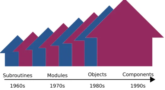
Component-based approaches are considered to be the current trend in developing modular software. It is set to be one level of abstraction higher thanobject-oriented programming(OOP) by promoting the separation of concerns. As it was noted that classes and objects in classical OOP techniques are not efficiently reused [Szyperski (2002)]. Component-based approaches are expected to be thede-factostandards among software engineers. Figure 2.3 shows a brief history of software progression towards higher levels of encapsulation and abstraction.

According to Szyperski (2002) the definition of a component is:

(12)

[image:12.595.149.423.82.232.2]

Figure 2.3: The trend of software development approaches towards further encapsulation and re-usability. Source: Northrop (2008).

Following the definition, a component is regarded as an executable unit which can be initial-ized, configured and deployed independently. It encapsulates computation and data, and in-teracts with the system only through predefined interfaces.

Software components follow a specific componentmeta-modelthat specifies its properties and internal structure. A great number of meta-models exist such as: CORBA [Wang et al. (2001)], BRICS [Bruyninckx et al. (2013)], Orocos [Bruyninckx (2011)], OPRoS [Song et al. (2008)], etc.

Component-based design(CBD) has its origins in different industries other than software, as it is heavily utilized in mechanical and electronics sectors, where a group of readily available component can be assembled into products. By avoiding the reinvention of components, CBD shortens the time-to-market of the product and improves maintainability. Hence, it is favorable as a design tactic in software. The adoption of CBD is advantageous not only in the industry but also in the research community as it allows researchers to focus on the core problem and avoid re-writing code.

2.3 Software product line

Software product lines(SPL) depicts a software engineering development paradigm which is used to create a family of applications that share a common set of functionalities. The main concept behind SPL is the identification of the stable and variable components within a group of applications in a specific domain. SPL then seeks to develop the components, the architec-tures and the tools in order to assemble the created software artifacts into a complete applica-tion.

Such a development methodology has been employed in many engineering fields such as au-tomotive, consumer electronics, avionics, etc. It has shown to improve the productivity and decrease the time-to-market of the products. Therefore, it is worthwhile to investigate product lines within the context of software engineering as it allows the developers to systematically and effectively reuse existing components, leading to mass customization of the software products [Gorton (2011)].

Software product lines have been successfully applied in many fields as listed in the SPLhall of fame3.

(13)

CHAPTER 2. BACKGROUND 7

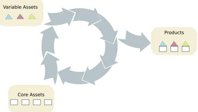
[image:13.595.144.465.118.299.2]

The primary concept of the product line development is visualized in Fig. 2.4, where the core and variable assets are identified, developed and assembled to create a family of applications.

Figure 2.4:Software product line approach; the core and the variable assets are developed and

(14)

3 Analysis

Considering the research objective stated in Chapter 1, the analysis aims at investigating the key concepts. Starting with the criteria that qualifies a software asset to become reusable. In addition to the common techniques and development paradigms in software engineering that promote reusability. Furthermore, this chapter provides a domain analysis regarding SLAM through surveying the fundamental components, the different strategies and the challenges in the current SLAM software implementations. Finally, an overview of the approach is given.

3.1 Reusability criteria

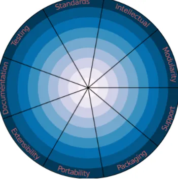
To develop reuse-oriented software, certain criteria have to be identified that will lead to a de-tailed description of software reusability. To this end, TheReuse Readiness Levels(RRLs) were introduced by Marshall et al. (2010) atNASA. Where 9 topics are presented as the main pillars that indicate the level of the reusability of a software product.

[image:14.595.197.373.390.568.2]

The 9 topics of the RRLs are visualized in Fig. 3.1. They are divided on a scale from 1 through 9 to match the commonly usedTechnological Readiness Levels(TRLs). A score of 1 means that the software is not recommended for reuse and 9 indicates that the software is supported and can be extensively reused. The following are the topics: documentation, extensibility, intel-lectual property issues, modularity, packaging, portability, standards compliance, support and verification & testing [Marshall et al. (2010)].

Figure 3.1:The 9 RRLs topics visualized along with the 9 levels per topic.

A highly reusable software will generally address all the mentioned RRLs. However, this work only considers the following topics due to timing constraints.

• Modularity: The degree of encapsulation and segregation of software modules.

• Standard Compliance: Following best practices and keeping the software modules co-herent.

• Extensibility: The ability of the system to grow past its current capabilities.

(15)

CHAPTER 3. ANALYSIS 9

There exist several software quality measures that can be applied such asISO25000 and the reusability metrics proposed in [Frakes and Terry (1996)]. However, the RRLs are chosen be-cause they are exhaustive and they regard reusability of the software as the main concern.

3.2 Challenges

This section highlights the main challenges that inhibit the reusability of the currently devel-oped SLAM software.

One of the most demanding obstacles to software reuse in SLAM is the tight coupling among the different components and the ill-defined interfaces which leads to unmaintainable

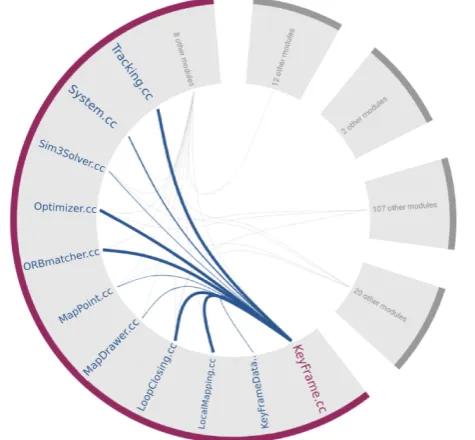
[image:15.595.184.422.356.576.2]

spaghetti code. Furthermore, most of the development is mainly concerned with showcasing a particular improvement or a novel algorithm in SLAM. Therefore, the implementation disre-gards the long term support of the product and focuses on the computational aspect alone. The source code in these cases would require extensive resources by experts to understand, mod-ify and extend [Brugali et al. (2012)]. The dense coupling can be clearly seen in Fig. 3.2 which shows the dependencies between one component and the rest of the system of a commonly used SLAM implementationORB-SLAM21. It can be seen that any changes to this component would trigger a chain of modifications to the majority of the system. In addition to the instance presented in Fig. 3.2, several examples showing architecture diagrams for a number of open-source SLAM implementations are available in Appendix A.

Figure 3.2:Function calls between a single component and the rest of the system in one of the

com-monly used SLAM open-source implementations2.

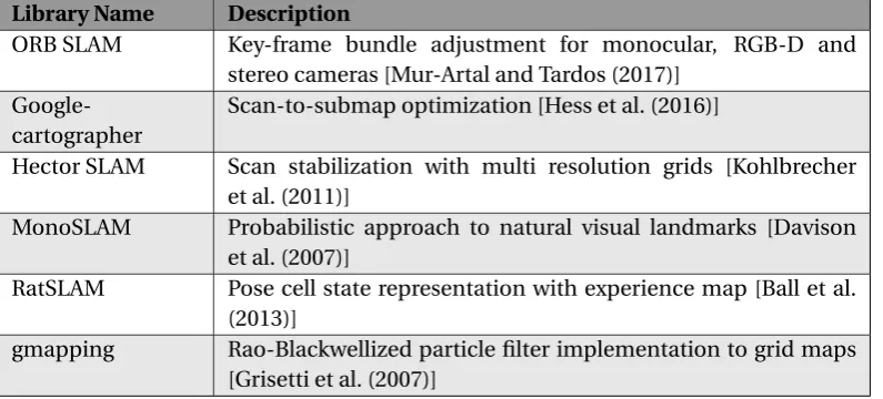
The challenges are exacerbated by the diversity and the rapid development of different SLAM algorithms which makes it a cumbersome task to evaluate, choose and integrate the suitable al-gorithm to a specific application. Moreover, SLAM is also customized to fit available hardware and middleware resources that leads to a suboptimal software realizations, where platform-specific features are hard-coded within the source code and entangled with computational parts. Table 3.1 shows a selection of commonly used SLAM implementations. More exten-sive lists can be found on different code repositories3, however, this collection only serves as a demonstration to the diversity of SLAM approaches.

1_{github.com/raulmur/ORB_SLAM2}

2_{The visualization is generated using}_{www.bettercodehub.com}

(16)

Library Name Description

ORB SLAM Key-frame bundle adjustment for monocular, RGB-D and stereo cameras [Mur-Artal and Tardos (2017)]

Google-cartographer

Scan-to-submap optimization [Hess et al. (2016)]

Hector SLAM Scan stabilization with multi resolution grids [Kohlbrecher et al. (2011)]

MonoSLAM Probabilistic approach to natural visual landmarks [Davison et al. (2007)]

RatSLAM Pose cell state representation with experience map [Ball et al. (2013)]

[image:16.595.89.487.80.260.2]

gmapping Rao-Blackwellized particle filter implementation to grid maps [Grisetti et al. (2007)]

Table 3.1:A number of open-source SLAM implementations using various approaches.

Moreover, The lack of a formal development methodology leads to an undesirable diversity in the software implementations; including data representations, interfaces and system architec-tures. The diversity hinders the interchangeability of the different implementations.

3.3 Reuse-oriented software development paradigms

After identifying the criteria of a reusable software and the shortcomings in the current SLAM development process, different paradigms from software engineering can be introduced in or-der to overcome the aforementioned challenges as they have been proven, tested and perfected over time. A number of development paradigms that promote reusability already exist such as component-based design, service-oriented design, layered-oriented approach, pipe and filter architecture, design patterns, software product lines, aspect-oriented architecture and many more.

The Software product line(SPL) approach has been proven to improve the software quality and decrease the development and deployment time of certain applications, provided that the applications share some commonalities. Additionally, SPL is often suited for growth scenarios where extra features, updates or modifications can be easily realized. The SPL approach has been applied successfully in many industrial sectors, furthermore, it has already been applied to the field of robotics by developing a reuse-oriented robot navigation [Brugali et al. (2012)].

As a complementary paradigm to SPL, Bruyninckx et al. (2013) provides best practices for de-veloping robotics software components based on theseparation of concerns”5C’s”, which pro-motes the splitting of 5 key aspects of a software artifact, namely, computation, communica-tion, configuracommunica-tion, coordination and composition.

3.4 Domain analysis

This section describes the domain analysis regarding SLAM in order to explore the different approaches and identify the fundamental components.

3.4.1 SLAM front-end

(17)

• Allothetic Information Unit: Which is responsible for the all the data processing for ex-teroceptive sensors that include: laser scanners (LiDARs), monocular cameras, RGB-D cameras, RADAR systems, etc. Two main operations are identified:

– Landmark Extraction: The operation tries to identify distinguishable landmarks from the raw sensor data which could be depth or visual data. The output is the detected landmarks which can be expressed by rangerand headingφ relative to the sensor’s reference frame. Considering the simple case of 2D landmarks the de-tections are expressed as [(r1,φ1), . . . , (rn,φn)]T for n detected landmarks. In the

case of visual data a large number of feature detectors can be employed such as

FAST,SURF,MSER,fiducial markers, etc. Tuytelaars and Mikolajczyk (2008) offers a survey over the commonly used visual feature detectors including scale, rotation and illumination invariant detectors. Additionally, depth data can be processed in a similar fashion in order to extract the landmarks. Edge detectors andRANSACare often used to extract corners and line segments respectively, moreover, G. Tipaldi (2010) proposescurvatureandblobdetectors for 2D laser scan.

– Data Association: The operation attempts to findcorrespondencesbetween the cur-rent observation and the already existing map. Considering the case of sparse land-marks, the matching occurs betweenkpreviously saved landmarks and the current

ndetections. The matching process is done according to different criteria such as:

euclidean distanceandlandmark descriptor. Moreover, association can be used to match raw measurements such as laserscan matchingandimage registration. • Idiothetic Information Unit: Which is responsible for converting the raw data from wheel

encoders, inertial measurement units, cameras (for visual odometry) etc. into motion commands that can be processed by the back-end.

The front-end often includes additional data processing such as noise removal, temporal alignment, coordinate transformation, scaling, etc. These tasks are essential during the pre-processing of sensor data [Cadena et al. (2016)].

3.4.2 SLAM back-end

The back-end of SLAM is described as the computational module responsible for the higher level processing of semantically sound information. It infers the states of the robot and the map of the environment given idiothetic and allothetic information. The back-end of SLAM is the abstract information processing unit which has seen several taxonomies and classifications across the literature. The three main identified approaches are:

1. The filter-based approach which is considered to be the classical and a popular tech-nique for SLAM. It maintains a probability distribution over the states of the robot as well as the map representation. A few examples are:extended Kalman filter(EKF),sparse ex-tended information filter (SEIF),particle filter(PF),unscented Kalman filter(UKF), etc. Chapter 2 presents the basic intuition behind this strategy. The filter-based approach is derived based on the recursive Bayes filter formulation which is briefly described as follows:

Considering that the required variables to be estimated arextand the mapmgiven

idio-thetic and alloidio-thetic information asutandztrespectively. Bayes rulecan be formulated

in Eq. 3.1, where the conditional probability is broken down into as the product of prior distribution, the measurement likelihood function and a normalizing factorη.

(18)

By applying theMarkovassumption and thelaw of total probabilitythe expression can be formulated in a recursive form. Where,ut andzt are considered to be conditionally

independentfrom one another and from past values.

p(xt,m|zt,ut)=η

upd at e

z }| {

p(zt|xt,m)

Z

xt−1

pr ed i c t

z }| {

p(xt|xt−1,ut)p(xt−1,m|z1:t−1,u1:t−1)

| {z }

r ecur si ve t er m

dxt−1 (3.2)

[image:18.595.120.450.332.418.2]

Equation 3.2 is considered to be the general expression for therecursive Bayes filter. The implementation of the update and predict expressions is dependent on the type of fil-ter, the robot, the map representation and the sensor. However, in all realizations the prediction encodes the motion and propagate the probability density function through a motion model, while the update takes into account the allothetic information and cor-rects the prediction estimate. It should be noted that the map termmis missing from the predict term due to the static map assumption. i.e. the environment is not affected by the robot motion [Mullane et al. (2008)].

Figure 3.3 presents the main building blocks of the filter-based approach showing the distinction between the front-end and the back-end.

Figure 3.3:Basic building blocks of filter-based SLAM algorithms and the information flow.

2. The optimization-based approaches formulate SLAM as a non-linear optimization prob-lem. The underlying structure can be interpreted as a graph representation, where the

nodesin the graph encodes the robot poses and the location of the landmarks. The nodes are linked by two types ofconstraints(edges); firstly, therelative motion constraintsthat link the different poses of the robot expressing idiothetic information. Secondly, the rela-tive measurements constraintsthat link the poses of the robot with landmarks in the map expressing allothetic information. Solving the optimization problem yields the optimal set of posesx∗and mapm∗such that the squared error of the constraints is minimized [Siciliano and Khatib (2016)].

The approach is used in many of the dominant SLAM implementation such as [Mur-Artal and Tardos (2017)] which runs the optimization problem on a number of key frames captured by vision sensors (also known asbundle adjustment). Furthermore, [Strasdat et al. (2010)] shows that optimization-based approaches outperforms classical filtering techniques in most cases.

3. Neural network-based approaches make use of the dynamics of Continuous Attractor Networks(CAN) in order to describe the motion and measurement updates. The states of the robots are represented as pose cells and the environment as an experience map. Ball et al. (2013) provides an open-source implementation for theRatSLAM which has successfully been utilized to map a suburban area using a single camera.

(19)

Although the underlying strategy for each of the aforementioned approaches is different, the interfaces are still comparable. The back-end requires idiothetic and allothetic information in order to generate the estimated the robot pose and the map.

3.4.3 Models

Models are considered to be sub-components utilized in both the front and the back-ends. The models encode the robot kinematics and the properties of the sensors along with their uncertainties. They are classified intomotionandmeasurementmodels.

• The motion model encodes the kinematics of the robot. Within the probabilistic context, motion models accepts as input idiothetic information generated from encoder data, ve-locity commands, IMU data, etc. And converts it into a probability density representation of the predicted robot pose, given the robot kinematics (state transition function), the previous pose and the process noise. The most commonly used models are thevelocity modeland theodometry model[Thrun et al. (2005)].

• The measurement model encodes the properties of the depth or vision sensors. Within the probabilistic context, measurement models accept allothetic information such as de-tected landmarks or laser scans and calculates the likelihood of an observation given the robot pose, the map and the noise characteristics of the sensor. The commonly used models arelikelihood fieldandrange-bearingmodels [Thrun et al. (2005)].

3.4.4 Additional modules

The aforementioned elements are fundamental to perform SLAM. However, a number of addi-tional funcaddi-tionalities could be implemented to further process the output of SLAM such as:

• Semantic Mapping: Is used to Provide a higher-level of understanding of the environ-ment. It can be briefly described as a categorization problem that tries to match semantic information to specific parts of the map allowing the system to add labels to these parts such as rooms, doors, corridors, etc [Cadena et al. (2016)].

• Scene reconstruction: Is used to render a dense point cloud representation of the envi-ronment. Which can be utilized in many different applications such as virtual or aug-mented reality. The image reconstruction functionality requires a sequence of images capturing overlapping areas in the scene along corresponding camera pose [Mur-Artal and Tardos (2017)]. This can be easily achieved by using the trajectory of the robot and the point clouds available in the map generated by SLAM.

• Volumetric map visualization: Utilizes depth data in order to obtain a semi-dense visu-alization of the environment. For example, a 2D floor plan can be obtained using a laser scanner. Each measurement is inserted into the map according to the current robot pose which is estimated by the back-end of SLAM.

• Path planning foractive SLAM: Is used to generate the trajectory that the robot should follow in order to improve the localization and the map estimates.

(20)

3.5 Approach overview

The analysis presents well-defined criteria for reuse-oriented software along with the develop-ment approaches and design tactics that achieve the identified requiredevelop-ments. It also shows that SLAM - although very diverse - has some stable components and interfaces which are always needed in order to correctly preform localization and mapping [Siciliano and Khatib (2016)]. The identified commonalities are considered to be well-suited candidates for decoupling and reuse; as they need not be designed and developed from scratch.

To this end,component-based designaugmented with thesoftware product lineapproach and theseparation of concernsare proposed as a development methodology to SLAM.

(21)

15

4 SLAM Framework Design

This chapter details the proposed methodology in 3.5 in order to create a reuse-oriented SLAM framework. The methodology is based on software product lines, component-based approach and the separation of concerns.

4.1 Feature model

[image:21.595.107.502.315.732.2]

Thefeature modelis set to be the first step in developing a software product line for a certain application. Figure 4.1 shows the developed feature model for SLAM. The model is considered as a graphical representation for the domain analysis performed in 3.4 as it identifies stable and optional functionalities. Mandatory functionalities are identified with a black circle notation at the link and optional functionalities with a white circle notation. Furthermore, a certain functionality can have different implementations which is represented as a variation point. The cardinality at the variation points specify if the alternative implementations are mutually exclusive ([1..1]) or inclusive ([1..∗]) [Badger et al. (2016)].

Figure 4.1:A feature model using theHyperFlextool-chain to identify the higher level stable

(22)

The model incorporates the front-end which is split into allothetic and idiothetic information units, the back-end as the information processing and the models which are commonly used in the front and the back-ends. The aforementioned elements are considered to be stable SLAM functionalities [Siciliano and Khatib (2016)]. Furthermore, a number of optional features are listed in the model.

Each functionality is detailed further according to the various implementations discussed in the domain analysis 3.4.

The developed feature model is by no means exhaustive nor definitive, however, it demon-strates the possibility of applying SPL to SLAM. Additionally, it does not include the variation points at the realization phase. Such as sensor configuration, middleware, communication protocols and the robotic platform used.

4.2 Software design

The feature model splits SLAM into functional blocks which are translated into software com-ponents and considered asprimitivesbuilding blocks (as described in Chapter 5). The com-bination of a number of components is labeled ascomposites. Finally, the integration of com-patible components into a working SLAM realization is considered as the finalapplications

[Kraetzschmar et al. (2010)]. The gradual construction strategy of components, composites and applications is chosen to ensure standalone deployment and extensive testing before reaching the final product.

4.2.1 Component level design

Acomponentis a piece of software that implements a certain functionality within SLAM1. From the practical point of view, a component is a group of classes that are managed by a component coordinator. The coordinator also offers the main entry point to the component and manages its public interfaces.

The following are the proposed requirements for each component in order to comply with the reusability criteria (RRLs) :

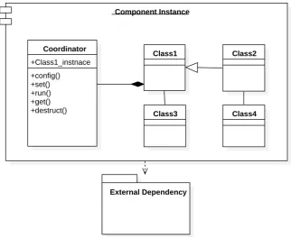
• A component as an entity should be treated as a black box with public interfaces to ensure information encapsulation as shown in Fig. 4.2.

Figure 4.2:An abstract representation of a component that encapsulates all the internal computation

and variables. It is only accessible through public interfaces.

• A component’s main entry point is the coordinator (also known as the mediator or the manager) which handles the creation, configuration, interfaces and destruction of the component. This can be considered partly as a mediator or a factory design pattern that

(23)

CHAPTER 4. SLAM FRAMEWORK DESIGN 17

[image:23.595.140.463.164.427.2]

inherently promotes loose coupling. Hence, Modification to the internal classes of the component can occur without the need to change the generic public interfaces of the coordinator such asconfigure()orrun()functionalities. An instance of a generic component is shown in Fig. 4.3. This design choice is in-line with the best practices pro-vided by Bruyninckx et al. (2013) in the BIRCS component model, where each component includes a coordinator.

Figure 4.3:An instance of a component as a group of classes that are managed by a coordinator which

is also the main entry point to the component’s functionalities. Different relationships bind the classes together, such as inheritance, composition and association. Furthermore, the external dependencies are specified explicitly.

• A component should be deployable standalone without dependency on other compo-nents. This property is considered to be a cornerstone in the component-based develop-ment approaches [Szyperski (2002)] (In contrary with common open-source implemen-tations of SLAM that offer a single executable entity).

• Within the boundaries of each component the separation of concerns should be followed as a best practice [Bruyninckx et al. (2013)]. The separation of the coordination, com-munication and composition is achieved by introducing the coordinator (The separa-tion could also be done within the middleware). Addisepara-tionally, the segregasepara-tion between the computation and the configuration is achieved by assigning the parameter values through external files at deployment-time.

• The component should be middleware independent. Nonetheless, wrapping into a spe-cific middleware such as ROS or Orocos can be achieved with minimal glue code. This is favorable to avoid major changes if a different middleware is chosen in future imple-mentations.

(24)

4.2.2 System level design

The system-level design introduces the structure of the system and the approaches used to compose the developed components. Two composition strategies are proposed in order to retain component segregation:

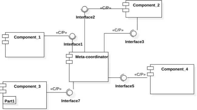
• A higher level coordinator (meta-coordinator) is used to build the complete application. It interfaces with all the different components’ coordinators through acaller/provider

«C/P»communication [Brambilla et al. (2012)]. The meta-coordinator is wrapped by

[image:24.595.123.448.250.431.2]

the middleware in order to communicate with the sensors. This centralized architecture highlights components segregation, consequently, any addition / modification / removal of a component will only be reflected in the meta-coordinator. The proposed structure is shown in Fig. 4.4.

Figure 4.4:Components composition through the meta-coordinator to deploy a complete application.

The centralized approach allows components to be oblivious to one another.

• Wrapping each of the individual components within the middleware such as ROS, allow-ing the components to communicate onpublish-subscribe«P/S»basis as show in Fig. 4.5. Such composition exploits the distributed nature of the middleware; also any addi-tion / modificaaddi-tion / removal of component will only affect the corresponding wrapper.

[image:24.595.122.446.548.695.2]

(25)

19

5 Components Development

This chapter describes the development of a number of components used to deploy SLAM ac-cording to the methodology defined in Chapter 4.

The derivation of a product from the software product line starts by selecting the constituting components. The selection is constrained by a set of rules defined by the developer to indicate that not all components combinations are valid. For example, non-parametric state represen-tation can not be used with an EKF back-end.

Following the feature model shown in Fig. 4.1 several components will be developed in order to serve as building blocks to deploy multiple SLAM instances. Figure 5.1 highlights the devel-oped components within the feature model. It should be noted that not all the components are deployed in a single instance as some of the selected blocks are mutually exclusive such as the EKF and the PF. Therefore, the figure only serves as road-map indicating the classification of the developed components.

The software framework is developed usingC++and a number of external libraries, namely,

[image:25.595.137.465.337.685.2]

OpenCV1,ArUco2andMRPT3.

Figure 5.1:Instance view inHyperFlexafter selecting the components required to perform SLAM based

on extended Kalman filter (EKF).

1_{http://opencv.org/}

2_{https://www.uco.es/investiga/grupos/ava/node/26}

(26)

Within the boundaries of the components, the separation of concerns is applied by distributing the computation across a group of classes. The communication, configuration and composi-tion is done by means of a component coordinator. Configuracomposi-tion is handled through separate files that are parsed during deployment-time.

5.1 Extended Kalman filter for feature-based map

Extended Kalman filter(EKF) is considered to be at the core of the earliest SLAM implementa-tion in Smith ’ et al. (1987). EKF realizes the recursive Bayes equaimplementa-tion in Eq. 3.2 by maintaining a parametric Gaussian representation over all the states including the detected landmarks in the form of a state vectorxtand a covariance matrixΣt[Thrun et al. (2005)].

The exchange of data to and from the component is done through the main interfaces shown in Fig. 5.2. It accepts idiothetic informationut representing odometry measurements. which

is used to propagate the states and the covariance matrix through the motion model; the result is the predictionp(xt|ut,xt−1). The landmarks are assumed to be static, therefore, the motion

does not affect their locations. Furthermore, the component processes the measurement vec-torzt containing the ranger and the bearingφobserved landmarks at timet along with their

associatedi d. new landmarks are appended to the state vector and previously seen landmarks are used to update the corresponding entries in the state vector and the covariance matrix.

The output is the estimated robot pose [x,y,θ]T and the landmarks in the environment repre-sented by their 2D coordinates (mx,my).

The motion and measurement models used in the EKF implementation are discussed in 5.3.

Figure 5.2:An abstract view of the developed EKF component with the main interfaces.

5.2 Fiducial marker detector

(27)

CHAPTER 5. COMPONENTS DEVELOPMENT 21

Figure 5.3: Fiducial marker detection using OpenCV ArUco module. The detected markers are

high-lighted.

5.3 Models

In order to encode the kinematics and the properties of the sensors along with their uncer-tainties, a probabilistic odometry motion model and range-bearing measurement model are developed for a 2D mobile robot mapping an environment populated with 2D landmarks.

5.3.1 Odometry motion model

The odometry motion model is used to calculate the predicted robot posep(xt|xt−1,ut) in the

recursive Bayes equation presented in 3.2. The input consists of incremental odometry values for translation and rotation4 ut =( ˆδt r ans, ˆδr ot)T that corresponds to the motion of the robot.

The (ˆ.) notation indicates that the odometry is noisy. The noise is assumed to be additive Gaus-sian noise with zero-mean expressed as²t r ansand²r otadded to each of the measurements.

The odometry increments are expressed relative to the robot’s local coordinate frame, there-fore, the state transition function in Eq. 5.1 resolves the motion to obtain the pose w.r.t the global reference frame.

  x0 y0 θ0  =   x y θ  +    ˆ

δt r anscos(θ+δˆr ot)

ˆ

δt r anssin(θ+δˆr ot)

ˆ δr ot





 (5.1)

Where, (x,y,θ)T is the robot’s previous pose and (x0,y0,θ0)T is the predicted pose.

Furthermore, in the case of an EKF back-end a linearized motion model is required in order to predict the covariance associated with the motion and to preserve the Gaussian assumption. A detailed derivation of the linearization is presented in [Thrun et al. (2005)].

The additive noise for the translation is expressed as²_α₁_δ2

t r ans+α2δ2r ot and for the rotation as

²α3δ2t r ans+α4δ2r ot. Where, ²is a Gaussian distribution with variance specified in the subscript.

Equation 5.2 simply formulates the addition of the noise terms.

The model offersα1, . . . ,α4 as process noise parameters that can be tuned according to the

robot platform used. The parameters can be described as follows:

• α1relates the translational motion to the uncertainty in translation estimate.

• α2relates the rotational motion to the uncertainty in translation estimate.

• α3relates the translational motion to the uncertainty in rotation estimate.

• α4relates the rotational motion to the uncertainty in rotation estimate.

4_{An extra rotation term}_δ

r ot2is occasionally added to the formulation which assumes that the robot performs an

(28)

·δˆ

t r ans

ˆ δr ot

¸

=

"

δt r ans+²_α₁_δ2

t r ans+α2δ2r ot

δr ot+²_α₃_δ2

t r ans+α4δ2r ot

#

(5.2)

5.3.2 Range-bearing model

The range-bearing model is implemented for 2D landmarks, where the model is used to cal-culate the likelihood of a certain measurement given the robot pose and the mapp(zt|xt,m),

which is the update term in the recursive Bayes formulation5presented in Eq. 3.2. For 2D land-marks the measurementzconsists of a rangeri and a headingφifor theit hlandmark and the model is formulated in Eq. 5.3 [Thrun et al. (2005)].

· ri φi ¸ = " q

(mxi−x)2+(miy−y)2

at an2((miy−y), (mix−x))−θ

#

+

"

²_σ2

r

²_σ2 φ #

(5.3)

Where, (x,y,θ)T is the robot pose, (mxi,miy)T is the world 2D coordinates for theit hlandmark,

(ri,φi)T is the estimated measurement and (²_σ2

r,²σ2_φ)

T _{is the assumed added Gaussian noise}

which has a zero mean and a variance ofσ2_randσ2_φfor the range and the bearing respectively. The noise parameters are sensor specific configuration values indicating the uncertainties in the measurements.

Furthermore, the inverse of the model is used to initialize the location of the landmarks, where the range and bearing are expressed w.r.t the sensor local frame and the landmarks needs to be initialized in the global frame. Therefore, Eq. 5.4 is used to initialize the landmarks location.

· mx my ¸ = · x y ¸ + ·

cos(θ) −si n(θ)

si n(θ) cos(θ) ¸ · xsens ysens ¸ +r ·

cos(θ+φ)

si n(θ+φ) ¸

(5.4)

Where, (x,y,θ)T is the robot pose, (xsens,ysens)Tis the sensor’s pose w.r.t the robot’s local frame

of reference and (r,φ)T is the range and bearing of a landmark w.r.t the sensor’s reference frame [Thrun et al. (2005)]. Figure 5.4 illustrates the different variables in Eq. 5.4.

5.4 Particle filter for feature-based map

The developed component for particle filtering is based on theRao-Blackwellizedparticle filter also known asFastSLAM[Thrun et al. (2005)]. The particle filter represents the robot pose through a set of weighted particles. The clustering of the particles at a certain location in the state space is proportional to the probability of the robot being in that state. Each particle maintains an independent estimate of the robot’s path andN extended Kalman filters (EKFs) over theN landmarks as shown in Eq. 5.5.

p ar t i cl e1={(x,y,θ)T}1_1:_t (µ1₁,Σ1₁) (µ1₂,Σ₂1) . . . (µ1_N,Σ1_N)

p ar t i cl e2={(x,y,θ)T}2_1:_t (µ2₁,Σ2₁) (µ2₂,Σ₂2) . . . (µ2_N,Σ2_N) ..

.

p ar t i cl eM={(x,y,θ)T}M_1:_t (µM₁ ,Σ₁M) (µ₂M,Σ₂M) . . . (µM_N,ΣM_N)

(5.5)

5_{the map}_m_{is considered to be a part of the state vector}_x_{in the EKF formulation and the measurement update}

(29)

Figure 5.4:.

In similarity to the previously developed EKF, the particle filter component accepts idiothetic informationut representing odometry measurements. which is used to propagate all the

[image:29.595.179.426.76.305.2]

par-ticles through the motion model. Furthermore, the particle filter uses the likelihood of the landmarks observations to calculate theweightfor each particle. Finally, the particles are re-sampledproportional to their weights. The re-sampling achieves the update step since the unlikely particles are eliminated from the new set of particles. The output consists of the robot pose and the detected landmarks according to the most likely particle (highest weight). Figure 5.5 shows the main interfaces.

Figure 5.5:The main interfaces of the particle filter component. It accepts odometry increments and

range-bearing measurements. The output is the estimated robot pose and the feature-based map ac-cording to the most likely particle.

5.5 Visual odometry

Visual odometry refers to the process of calculating the incremental translation and rotation of the robot using a sequence of images. In this approach, SURF Keypointsare detected in two subsequent frames along with their descriptors. The descriptors are used to find matches between the two frames, afterwards a variant ofRANSACis used for outliers rejection. The re-maining matches are used to calculate asimilarity transformationbetween the two frames. The transformation encodes the relative translation and rotation (δt r ans,δr ot). The visual

(30)

odometry algorithms can be used such asKLT trackers [Fraundorfer and Scaramuzza (2012)] anddeep convolutional neural networks[dee (2016)].

Figure 5.6:Keypoints matching between two consecutive frames captured by an upward looking

cam-era.

5.6 Point-map visualization

A Point-map visualization component represents the environment as a 2D floor plan with each point in the map corresponding to an object detected by the laser scanner (different ranging sensors can be used). The developed component accepts 2D laser scan data as input along with the estimated robot pose. Each range data is transformed into the global frame in similarity to Eq. 5.4 and compared with each existing point in the map. Euclidean distance is compared against a threshold to determine whether the range measurement is fused with the current map or appended to it.

As an additional component, the point-map visualization has no effect over the pose estimate nor the map within the back-end of SLAM.

[image:30.595.126.421.123.319.2]

The component interfaces and the sample visualization are shown in Fig. 5.7.

Figure 5.7:Point-map visualization component along with the main interfaces. The components

(31)

5.7 Particle filter for grid-based map

Occupancy grid maps are often favored over feature-based maps as they do not require an ex-plicit definition of the landmarks and could offer a more informative representation of the en-vironment [Grisetti et al. (2007)]. Occupancy grid maps discretize the enen-vironment into a finite number of cells each carrying a probability value indicating if the cell is considered as free-space or occupied.

The previously developed particle filter can be extended to handle occupancy grid maps by adapting the calculation of the likelihood function that computes the likelihood of a certain measurement based on the pose of the particle and its corresponding grid mapp(zt|xi_t,mi) for theit h-particle. Similarly to the feature-based map, the likelihood is used to update the weight of each particle. Figure 5.8 shows the list of particles, where each particle consists of a robot path and an independent map.

Furthermore, the grid map for each particle is updated through calculating a posterior func-tion for each grid cell j within the mapp(mi_j|zt,xit) in order to obtain the full map posterior

[image:31.595.159.445.315.477.2]

p(mi|zt,xi_t) for theit hparticle. The detailed derivation is presented in [Thrun et al. (2005)].

Figure 5.8: Particle list for grid-based maps. Each particle maintains a separate occupancy grid that

(32)

6 Evaluation

The results and the evaluation of the proposed framework is presented in this chapter along with the experimental design and the hardware information.

The evaluation consists of two aspects; firstly, the derivation of several use-cases from the prod-uct line is assessed from the reusability point of view according to the RRLs discussed in 3.1. The evaluation will adopt the concept of scenarios fromATAMin order to come up with quan-titative measures for the chosen RRLs, namely, modularity, extensibility, standards compliance (5Cs) and testing & verification.

A number ofuse-caseandgrowthscenarios are created in order to evaluate each of the chosen RRLs. A summary is presented in Table 6.1.

Target RRLs Modularity Extensibility Testing Standards

Scenarios

Component replacement +++ ++

Component addition +++ +

Logic modification ++ ++

Standalone deployment ++ +++

Deployment-time configuration + +++

Table 6.1:A general description of the proposed scenarios and the target RRL to be evaluated

accord-ingly.

In each of the scenarios mentioned in 6.1 a quantitaive measure will be given based on:

• The number of replaced / added / modified components

• The number of replaced / added / modified interfaces

The second aspect of the evaluation is the performance of the different SLAM realizations. A qualitative measure is proposed based on the ability to generate a consistent path and map estimation during the presence of multiple loop-closures i.e. ability to close the loop and cor-rectly recognize previously visited location, which is considered to be the differentiating factor between SLAM and plain odometry [Cadena et al. (2016)], therefore, it is considered as a de-factocriterion to assess SLAM systems.

6.1 Experimental setup

A Segway RMP 50 omni-directional platform is used to run the experiments; it can be controlled through on-board intel NUC. The platform is tele-operated using a Logitech extreme 3D pro joystick. The sensors used are:

• Kinect for XBOX-360 (Only RGB camera is used).

• Hokuyo LiDAR urg-04lx-ug01.

• Upward-looking camera Logitech HD C615 webcam.

• Segway RMP 50 built-in wheel encoders.

(33)

CHAPTER 6. EVALUATION 27

6.2 SLAM deployment

This section describes the deployment of 5 different SLAM realizations. The different instances will be used to estimate the robot path and the map for a relatively small indoor office envi-ronment (≈10m2) using the same dataset. The environment is randomly populated with fidu-cial markers and the robot is manually driven in approximately the same trajectory twice to evaluate loop-closure capabilities. The dataset does not include ground truth measurements, therefore, no quantitative evaluation of SLAM is provided.

The developed components are composed according to the system architecture proposed in Fig. 4.4, where a meta-coordinator instantiates and communicates with the different compo-nents through acaller/providercommunication (highlighted as«C/P»). Furthermore, it inter-faces with the sensors using ROS throughpublisher/subscribercommunication (highlighted as

«P/S»). The alternative system composition strategy proposed in Fig. 4.5 is not implemented due to time constraints.

6.2.1 Extended Kalman filter feature-based SLAM

[image:33.595.142.464.370.509.2]

The component diagram shown in Fig. 6.1 presents the integration of a number of selected components from the feature model in Fig. 5.1. The application uses wheel odometry as an id-iothetic information source and a front camera to detect fiducial markers as the source for allo-thetic information. The back-end is based on an extended Kalman filter that includes odometry and range-bearing models.

Figure 6.1:EKF feature-based SLAM component diagram.

Figure 6.2a shows the path and the map generated from SLAM instance described in 6.1 using the defined dataset.

Figure 6.2b is presented in order to highlight the differences between the path estimate gen-erated by SLAM and by dead reckoning which is based solely on wheel encoders (idiothetic information). The error accumulation in dead reckoning produces an inconsistent path as the second loop trajectory clearly does not align with the first one, while in the case of SLAM, ex-ternal landmarks (allothetic information) are used to correct for the drift in odometry and gen-erate a more consistent path.

6.2.2 Particle filter feature-based SLAM

(34)

par--2 0 2 4 6 8 10 X direction [m]

-6 -4 -2 0 2 4

Y direction [m]

Path Landmarks

(a)EKF feature-based SLAM trajectory

estima-tion along with the detected landmarks and the corresponding error ellipses.

-2 0 2 4 6 8 10 X direction [m]

-5 -4 -3 -2 -1 0 1 2 3 4 5

Y direction [m]

Wheel odometry

(b)Dead reckoning using only wheel encoders.

[image:34.595.301.482.86.228.2]

The error accumulation leads to an inconsistent trajectory estimation.

Figure 6.2:Robot’s path estimation using EKF SLAM and dead reckoning.

[image:34.595.84.270.89.229.2]

ticle filter component. The interfaces are identical as the particle filter implements a feature-based map and processes the same motion and observation data.

Figure 6.3:Particle filter feature-based SLAM component diagram.

Figure 6.4 shows the estimated path and map using the particle filter. The estimates are slightly more consistent compared to the EKF results in Fig. 6.2a.

6.2.3 Visual odometry-based SLAM

A visual odometry component is used to replace the wheel encoders. Figure 6.5 shows the corresponding component diagram highlighting the replacement of wheel encoders by a visual odometry component and the addition of an upward-looking camera along with two interfaces to receive the image data from the camera and pass it to the visual odomerty component.

The results in Fig. 6.6b show that both odometry techniques suffer from drift, however, the visual odometry results in a relatively more consistent path estimation compared to the wheel encoders. It is also noted that the error accumulation in both techniques is not identical as it introduces different biases leading to a slightly rotated version of the trajectory.

[image:34.595.121.450.365.499.2]

(35)

-2 0 2 4 6 8 10

X direction [m]

-4 -2 0 2 4 6

Y direction [m]

[image:35.595.179.426.93.281.2]

Path Landmarks

Figure 6.4:Particle filter feature-based SLAM path estimation along with the detected landmarks and

[image:35.595.140.467.356.492.2]

their corresponding uncertainty ellipses.

Figure 6.5:Wheel encoders replaced by visual odometry in the particle filter SLAM instance.

-2 0 2 4 6 8 10 12 14

X direction [m] -8

-6 -4 -2 0 2 4

Y direction [m]

Path Landmarks

(a)Particle filter path estimation with

feature-based maps using visual odometry.

-10 -5 0 5 10 15 20 X direction [m]

-5 0 5

Y direction [m]

Wheel Odometry

-10 -5 0 5 10 15 20 X direction [m]

-5 0 5

Y direction [m]

Visual Odometry

(b)Visual odometry versus wheel odometry path

[image:35.595.320.494.551.692.2]

estimations.

(36)

6.2.4 Point-map visualization

[image:36.595.124.449.176.325.2]

A points map visualization component is added to the EKF SLAM realization in Fig. 6.1 as a part of component addition scenarios. Figure 6.7 shows the corresponding component dia-gram that describes the addition of a laser scanner and the additional visualization component along with their interfaces. The estimated pose by the EKF is used in the to the visualization component.

Figure 6.7:Points map visualization.

The generated points map is presented in Fig. 6.8 along with the EKF path estimate. The result shows an inconsistent map as the trajectory overlaps occupied areas at some parts of the map. However, the added map provides as relatively more intuitive description of the environment compared to the feature-based map.

-4 -2 0 2 4 6 8 10 12

X direction [m]

-8 -6 -4 -2 0 2 4

Y direction [m]

Points Map Path

Figure 6.8:Points map visualization.

6.2.5 Particle filter grid-based map

[image:36.595.126.415.436.659.2]

(37)

[image:37.595.140.466.83.239.2]

[image:37.595.99.441.336.619.2]

Figure 6.9:Modifying particle filter component to accommodate the addition of occupancy grid maps.

Figure 6.10 shows the generated occupancy grid map as a part of the particle filter along with the estimated robot trajectory and the detected landmarks. The result shows consistent path estimation as it aligns with the free spaces. The generated map is relatively consistent as well.

Figure 6.10:Occupancy grid map augmented with the estimated trajectory and the detected landmarks

(38)

6.3 Discussion

This section discusses the results according to two aspects as specified in the introduction of the chapter, namely, the evaluation of SLAM and the reusability scenarios.

6.3.1 Trajectory & map estimation

Figures 6.2a, 6.4, 6.6a and 6.10 show the results of running different SLAM realizations using the same dataset. The outcome consists of the robot’s path and the generated map of environment, where it can be seen that the different realizations were able to detect all the landmarks placed in the environment, estimate the path of the robot consistently, recover from odometry drift and perform loop-closures.

The volumetric map visualization component added to the EKF instance as shown in Fig. 6.7 did not yield a consistent map as the result indicates in Fig. 6.8. Due to the elementary fusion method employed that matches the map points based solely on euclidean distance. The map can be improved by using a more sophisticated technique such as scan-to-map optimization as Hess et al. (2016) proposed.

6.3.2 Use-case & growth scenarios

The component replacement scenario had two occurrences; the EKF was replaced with a par-ticle filter and the visual odometry was used instead of wheel encoders. In the first occurrence The replacement effects are confined to the meta-coordinator which had to simply be adapted to instantiate the PF component instead of the EKF as shown in Fig. 6.1. In the second scenario the meta-coordinator was modified to instantiate the visual odometry component and add two new interfaces to pass the image data as presented in Fig. 6.5. The fact that the replacement did not have system-wide effects indicates thatmodularityas a first target RRL has been addressed. A component addition scenario was realized by adding a point-map visualization to the EKF SLAM. The meta-coordinator was simple modified to instantiate a points map component and pass the laser scan and pose information through the added interfaces as shown in Fig. 6.7. An additional growth scenario is implemented by extending the particle filter to accommodate a grid map representation. Figure 6.9 shows the modifications in the particle filter component and the meta coordinator which is required to pass the laser scan data from the sensor to the filter.

The component addition and the logic modification indicates that the system is capable of growing beyond the current implementation without the need to rebuild the majority of the components to be adapted to the expansions, which implies that the system isextensible. Generally, the derivation of the developed components into a working SLAM instance in the previous scenarios required minimal glue code and integration time. The interfacing con-sists of approximately 6 function calls per component. The common operations offered by all components areconstruct(),configure(),set(. . .),execute(),get(. . .)and

destruct(). Additionally, the performance of each component is configured through a

sep-arate configuration file that is parsed at deployment-time with no need to modify or re-compile the source code. Therefore, the components are considered coherent and adhering to the spec-ified design patterns and the 5Cs, which improves thestandards complianceRRL.

(39)

[image:39.595.91.389.124.731.2]