warwick.ac.uk/lib-publications
A Thesis Submitted for the Degree of PhD at the University of Warwick
Permanent WRAP URL:
http://wrap.warwick.ac.uk/79699
Copyright and reuse:
This thesis is made available online and is protected by original copyright.
Please scroll down to view the document itself.
Please refer to the repository record for this item for information to help you to cite it.
Our policy information is available from the repository home page.
M A
O
D
C
S
Sample path large deviations for the
Laplacian model with pinning interaction
in
(1 + 1)
-dimension
by
Alexander Karl Kister
Thesis
Submitted for the degree of
Doctor of Philosophy
Mathematics Institute
The University of Warwick
Contents
Acknowledgments iii
Declarations iv
Abstract v
Chapter 1 Introduction 1
Chapter 2 Integrated random walk 18
2.1 Integrated random walk sample path large deviations . . . 18
2.2 Integrated random walk bridge sample path large deviations, with zero boundary condition . . . 21
2.3 Integrated random walk bridge sample path large deviations, non zero boundary condition . . . 27
2.4 Preparation for the proof of Theorem 1.3 . . . 29
2.4.1 Goodness of the rate function . . . 29
2.4.2 Extension of Theorem 1.2 . . . 31
2.4.3 Uniformity . . . 32
Chapter 3 Large deviation principle for the model with pinning in-teraction 35 3.1 Goodness of the rate function . . . 35
3.2 The large deviation principle for the model with pinning interaction 37 3.2.1 Lower bound . . . 38
3.2.2 Upper bound . . . 45
Chapter 4 Minimiser of the rate function of the model with pinning interaction 61 4.1 Superset of the set of minimisers . . . 62
4.3 With terminal condition . . . 83
4.3.1 Symmetric boundary condition wherea6= 0 and aα <0 . . . 87 4.3.2 Symmetric boundary condition wherea6= 0 and aα >0 . . . 93
4.3.3 Symmetric boundary condition withα= 0 . . . 94
4.3.4 Symmetric boundary condition witha= 0 . . . 94 4.3.5 Collection of remaining proofs . . . 95
4.3.6 Remarks on how to deal with general boundary conditions . . 98
Chapter 5 Outlook and conclusion 100
5.1 Concentration . . . 100 5.2 Wetting . . . 106
5.3 Conclusion . . . 109
Appendix A Large deviation theory 111
Appendix B Gaussian measure 114
Appendix C The partition function 116
Appendix D Minimisers of the rate function of the model without
pinning interaction and of the Hamiltonian 120
Acknowledgments
I would like to thank my supervisor Stefan Adams for introducing me to the topic
of this thesis and for his guidance throughout my studies. I also like to thank my
second supervisor Hendrik Weber for his help and support in writing this thesis.
Furthermore I like to thank Stefan Grosskinsky for joining some discussions at the
beginning of my PhD.
Next, I would like to thank all my departmental friends and all my flatmates
for their company during my time at the University of Warwick. Especially I like
to thank my good friend Amal Alphonse for his help in proofreading some parts of
this thesis. I also like to thank my parents, my sister and my grandmother for their
encouragement.
Finally, I would like to thank the Engineering and Physical Sciences Research
Council (EPSRC) for the funding they provide and everyone involved with the
Declarations
The work presented here is my own, except where specifically stated otherwise, and
was performed in the Department of Mathematics at the University of Warwick
under the supervision of Dr. Stefan Adams and Dr. Hendrik Weber. I confirm that
Abstract
We consider the (1+1) dimensional Laplacian model with pinning interaction.
This is a probabilistic model for a polymer or an interface that is attracted to the
zero line. Without the pinning interaction, the Laplacian model is a Gaussian field
(φi)i∈ΛN, where ΛN = {1,2, . . . , N −1}. The covariance matrix of this field is
given by the inverse of φ 7→ 12PN
i=0(∆φi) 2
, where ∆ is the discrete Laplacian.
Furthermore the values at{−1,0, N, N+ 1}are fixed boundary values. The pinning
interaction is introduced by giving the field a reward each time it touches the zero
line.
Depending on the reward the model with pinning and the one without
pin-ning show different behaviour. Caravenna and Deuschel [10] study the localisation
behaviour of the polymer. The model is delocalised if the number of times a typical
field touches the zero line is of ordero(N). The authors of [10] show that for zero
boundary conditions there is a critical reward such that for smaller rewards the
model is delocalised whilst for larger rewards the model is localised.
In this thesis we study the behaviour of the empirical profile of the field. We
show that for non zero boundary conditions there is a critical reward such that for
smaller rewards the empirical profile for the model with pinning and the one for
the model without pinning behave in the same way whilst for larger rewards the
Chapter 1
Introduction
Probability theory has been influenced by statistical physics for at least fifty years. The models that we study have their origin in statistical physics, too. In the
math-ematical literature they appear under the namesrandom interface (see [16, 21, 17])
orrandom polymer models (see [22, 9]). Mathematically those models are random fields, i.e. families of countably many random variables.
The models appear under different names because they are used to explain
different natural phenomena. A polymer is a long chain of repetitive units, called monomers. Random polymer models are designed to study the special arrangement
of the monomers. Interface models describe the surface between two coexisting
phases, for example, the one between water and ice at 0◦C or the one between areas of positive and negative magnetisation in a ferromagnet. The atoms forming the
surface are calledinterface. One approach to study these interfaces is to model the
complete system, for example a volume of water or a ferromagnet, see [15]; another way - and this is the one where our models emerged from - is to model only the
atoms that form the interface but such that this reduced model is still consistent
with a model of the full system. This second approach leads to so-called effective models. These models are called effective because they only describe the location of
the interface above a reference level and not the full system. The random interface
models are such effective models.
The goal of the polymer and interface models is to understand how these
systems interact with their environment. For example a polymer can be attracted
to a membrane; if the membrane is penetrable we call this interactionpinning and if the membrane is not penetrable we call the interactionwetting. Depending on the
We study models with so-called Laplacian interaction and compare our
re-sults to models with gradient interaction.
The Laplacian model with pinning interaction
Laplacian models with pinning interaction are random fields φ on Z. A random
field onZ is a family of real valued random variables indexed by a subset ofZ. To
define the distribution of the fieldφin the subset ΛN :={1,2, . . . N−1}we use the
functions
HN(φ) :=
1 2
N
X
i=0
(∆φi)2, (1.1)
whereN ∈Nand ∆ is the discrete Laplacian given by
∆φi:=φi−1−2φi+φi+1.
In physics, forN ≥2, the valueHN(φ) is called the total energy ofφin ΛN andHN
is the Hamiltonian in this set. The Hamiltonian models how the heights (φi)i∈ΛN
interact with each other and with the boundary (φi)i∈{−1,0,N,N+1}.
To understand the interaction let N = 2 and fix the boundary condition
(φi)i∈{−1,0,2,3}. So the only height which is not fixed isφ1. The heightφ1 is energet-ically optimal if it minimises the total energy under the given boundary condition.
The HamiltonianH2is the sum of the squares of the three Laplacians ∆φ0, ∆φ1and ∆φ2. Considering each of these terms separately, we see that it would be optimal ifφ1 is such that each of the heightsφ0, φ1 and φ2 coincides with the average of its neighbouring heights, because then each Laplacian would be zero. But for general boundary conditions (φi)i∈{−1,0,2,3} a φ1 that is such thatφ0 coincides with the av-erage of φ−1 and φ1 does not coincide with the average of φ0 and φ2. In general there is a trade off between choosing φ1 such that φ0 or φ1 or φ2 coincides with the average of its neighbouring heights. So φ1 interacts with its nearest and next nearest neighbours.
To define the fieldφwe need a boundary conditionψ∈RΛN , where the set
ΛN :={−1,0, . . . , N+1}. The field is given by the following probability distribution:
γNψ,J(dφ) := 1
ZNψ,Je − HN(φ)
N−1
Y
i=1
(dφi+eJδ0(dφi))
Y
i∈{−1,0,N,N+1}
δψi(dφi),
where dφi is the Lebesgue measure on R and δ0 is the Dirac measure at zero and
physics as the partition function
ZNψ,J :=
Z
RΛN
e− HN(φ)
N−1
Y
i=1
(dφi+eJδ0(dφi))
Y
i∈{−1,0,N,N+1}
δψi(dφi).
The terms eJδ0(dφi) attract φ to the zero line. Note that in physics the measure
γNψ,J is called the Gibbs distribution in ΛN with boundary conditionψ, interaction
potential (∆φi)2, and single spin measure (dφi+eJδ0(dφi) (see [20, Definition 2.9]).
To simplify the notation we use the conventions
γNψ :=γNψ,−∞, ZNψ :=ZNψ,−∞;
and in contexts whereJ >−∞is fixed we use the notation
ˆ
γNψ :=γNψ,J, ZˆNψ :=ZNψ,J.
Random walk representation
The random fields from above are related to a special class of random walks, the integrated random walks (IRWs). First we consider the case J = −∞. To define the IRW let X1, X2, . . . be a sequence of independent and identically dis-tributed (i.i.d.) standard normally disdis-tributed random variables on a probability space (Ω,E, Pψ); we call the processes (Yn)n∈N0 and (ζn)n∈N0 given by
Y0 =ψ0−ψ−1, Yn=Y0+
n
X
i=1
Xi, forn≥1; ζ0 =ψ0,ζn=ζ0+
n
X
i=0
Yi, forn≥1,
(1.2)
random walk and IRW, respectively. The laws of (ζi)i∈ΛN under the measure
PNψ(·) := Pψ(·|ζN = ψN,ζN+1 = ψN+1) and of (φN)i∈ΛN under the measure γ
ψ N
coincide. To see this we study their densities. The most important observation for this study is that if two random variables have the joint density f(x, y), then the density of the first random variable given that the second is zero coincides up to
a multiplicative constant with f(x, y)δ0(dy). So for zero boundary conditions it is enough to show that the density of the IRW under P0 is up to a multiplicative constant equal to
e− HN(φ)δ0(dζ
Since ∆ζi =Xi+1, we have for Y0 = 0 and ζ0 = 0 that
P0((∆ζ0,∆ζ1, . . . ,∆ζN−1,ζ−1,ζ0)∈(dx1,dx2, . . . ,dxN,dζ−1,dζ0))
=P0((X1, X2, . . . , XN,ζ−1,ζ0)∈(dx1,dx2, . . . ,dxN,dζ−1,dζ0))
= C1e−12
PN i=1x2i
N−1
Y
i=1 (dxi)
Y
i∈{−1,0}
δ0(dφi), (1.4)
whereC is a normalisation constant. Substitutingxi by ∆ζi−1 in the last equation we see that the density of the IRW under P0 is up to a multiplicative constant equal to (1.3). For the argument for non zero boundary conditions see [10, Lemma
2.1, Proposition 2.2].
For J > −∞ relating the random field and the IRW requires a different argument. Note that the reference measure has the expansion
Y
i∈ΛN
(dφ(i) +eJδ0(dφ(i))) =
X
S⊂ΛN
eJ|Sc| Y
i∈Sc
δ0(dφi)
Y
i∈S
(dφi), (1.5)
where we use the convention Sc := ΛN \S and where |S| is the cardinality of S.
Under the assumption thatψi = 0 for i∈ΛN, the expansion (1.5) implies that for
a setAthat is measurable with respect to theσ-algebra generated by{φi|i∈ΛN}
we have:
ˆ
γψN(A) = ˆ1
Zψ
X
S⊂ΛN
eJ|Sc|ZSψγSψ(A), (1.6)
where
γSψ(dφ) := 1
ZSψe
− HN(φ) Y
i∈S
(dφi)
Y
i∈Sc
δψi(dφi),
and
ZSψ :=
Z
RS
e− HN(φ) Y
i∈S
(dφi)
Y
i∈Sc
δψi(dφi).
A sample from γSψ coincides inP := Sc with ψ. We say the measure γSψ is pinned to ψ at the sites P. The measures γψPc are related to the IRW as follows:
analogously to (1.3) we see that the laws of (ζi)i∈ΛN under P
ψ(·|ζ
i = ψi, fori ∈
P ∪ {−1,0, N, N+ 1}) and of (φi)i∈ΛN underγ
ψ
Pc coincide.
The reason for namingγSψ not after the sites where the reference measure has
δmeasures but after the sitesSwhere the reference measure has Lebesgue measures is down to the fact that this is consistent with the definition ofγNψ: just letS = ΛN
and note thatγSψ =γNψ .
procedure:
Stage 1: Sample a subset ofP ⊂ΛN according to the law
eJ|P| Z ψ Pc
ˆ
ZNψ .
Stage 2: Sample an element ofRΛN according to the lawγPψc.
The IRW does not satisfy the Markov condition but it satisfies a Markov
condition with lag 2, which means that we need to know the current and the most recent past state in order to know the distribution of the future of the chain. For
the measuresγSψ and partition functions ZSψ this has the consequence that
γSψ =γψS
1γ
ψ S2
ZSψ =ZSψ
1Z
ψ
S2 (1.7)
ifS=S1∪S2 and minS2−maxS1 ≥3 (note that this implies that the gap between
S1andS2is at least two, but also note that also the setsS1andS2are not necessary connected). We call this the splitting property of lag 2.
The gradient model with pinning interaction
A related model is the gradient model (see [19]). This model differs from the Laplace
model only by the Hamiltonian; the gradient model is defined with the Hamiltonian
H∇N(φ) := 1 2
N−1
X
i=0
(∇φi)2, for Λ⊂Z,|Λ|<∞ (1.8)
where
∇φi :=φi+1−φi.
With this Hamiltonian, each height φi interacts only with its nearest neighbours.
We denote the probability distribution of the field with gradient interaction byγ∇N,ψ. For J =−∞, the law of the gradient model coincides with the law of the random walk under the condition thatY0 =ψ0 and YN =ψN. The gradient model satisfies
the splitting property (1.7) with lag 1, that means that (1.7) is satisfied already for
S=S1∪S2 such that minS2−maxS1 ≥2.
The random walk representation implies that for certain types of polymers,
the so-calledsemi-flexible polymers [8], the gradient model is a less suitable choice
gradients of the polymer are correlated. For the gradient model, where the gradients
areXi, this is clearly not the case while for the Laplacian model, where the gradients
are Yi, this is the case. A model that is related to the Laplacian model but also
captures other aspects of semi-flexible chains is studied in [24].
Localisation and delocalisation
For the Laplacian and the gradient model, we measure whether the reward has any
effect by the expected fraction of pinned sites:
EJ[|P|N ],
where we write EJ for the expectation with respect to the measure γN0,J, γN∇,0,J , respectively. A quantity related to that expectation is the pinning free energy; which is defined as
τ(J) := lim
N→∞τN(J), τN(J) :=
1
N log ZN0,J
Z0
N
. (1.9)
To see this relation note that by (1.5) we have
d
dJτN(J) =
1
ZN0,J
X
P⊂ΛN |P|
N e J|P|Z0
Pc = EJ[|P|/N].
So ifτ(J) is identical to zero in an interval (−∞, Jc], then, for largeN, the fraction
of pinned sites is almost surely zero for allJ ≤Jc. Ifτ(J)>0 , we call the model
with rewardJ localised and otherwise we call itdelocalised.
For the gradient model we haveτ(J) >0 for all J >−∞ (see [19, Remark 6.1]), while for the Laplacian model there is a Jc > −∞ such that τ(J) = 0 for
J ≤Jc and τ(J)>0 ifJ > Jc (see [10, Theorem 1.2]).
To prove that for the gradient model we have Jc = −∞ Funaki and
Saka-gawa [19] show that forN large enough there is a constantCsuch that the following inequality is true:
ZN0,J Z0
N
= X
P⊂ΛN
eJ|P|Z 0 Pc Z0
N
≥ X P⊂ΛN
eJ|P|e−C|P|= (1 +eJ−C)N−1. (1.10)
The argument for this inequality uses that since the gradient model satisfies the
splitting property with lag 1, the partition function Z0
Pc is a product of partition
functions of the form Z0
S whereS ={s∗+ 1, . . . , s
∗−1}=: (s∗, s∗) and that Z0
S =
Z0
|S|. Since for the gradient model theZN0 is equal to the square root of a polynomial
For the Laplacian model the splitting property is not satisfied with lag 1. To determine the critical reward Jc for the Laplacian model Caravenna and
Deuschel [10] consider only certain properties of the field ˆγN0: they consider the zero setP and heights before these zeros. To do so they use the density
ˆ
γN0(|P|=k,Pi=ti,dbi∈dyi, i∈ {1,2, . . . k}),
where P ={P1,P2, . . .Pk}, Pi <Pi+1, and bi are the values before the chain hits
zero:
bi :=φPi−1.
They represent (P, b) with the help of a Markov renewal process (see [1, Chapter VII 4]).
Using this representation Caravenna and Deuschel [10] prove in addition
to Jc > −∞ also some properties of the function J 7→ τ(J): For Jc < J < ∞
the function J 7→ τ(J) is real analytic with 0 < τ(J) < ∞ and for J → ∞,
τ(J) = J + log(1 +o(1)), see [10, Theorem 1.2]. They also show that the first derivative of the function J 7→ τ(J) at Jc is zero and that the second derivative
does not exist, see [10, Theorem 1.4]. In statistical physics such a transition with a
discontinuity in the second derivative is calledsecond order transition. Furthermore the authors of [10] consider the number of sites at which a typical path picks reward:
For J ≤ Jc this number is of order o(N) while for J > Jc this number increases
at least linearly in N. Additionally they show that for J > Jc the maximal gap
between sites at which a typical path picks reward is of ordero(N).
In the following lemma we quote a result that Caravenna and Deuschel [10]
obtain during their study of the free energy.
Lemma 1.1. For each J, there is a renewal processχ={χk}k∈N such that
ZN0,J Z0
N
= 2πpp(N)eτ(J)N−2JP(N + 1∈χ), (1.11)
where
p(N) = 16N +125 N2+13N3+121N4.
ForJ ≥Jc, the processχ is non terminating.
add (N+ 1) log(√2π) to our HamiltonianHN and because by Proposition C.1
ZN0 =
√
2πN−1
√
p(N) .
For a summary on the properties ofχsee [11, Section 3.1.].
Large deviations of the empirical profile
The following results concern empirical profiles. They are given with the help of
a functionhN:RΛN → C(0,1), where hN(φ) is the linear interpolation of a scaled
version of (φξN)ξ∈ΛN/N.
In this thesis we study for which reward level J the empirical profile of the Laplacian model with pinning behaves different than the one of the Laplacian
model without pinning (J =−∞). Furthermore we investigate the influence of the boundary condition on this critical rewardJ. Intuitively it is clear that for non zero boundary conditions the critical reward is larger than Jc, because if the interface
does not start in zero it has to go down or up before it can touch zero.
To study the effect of the pinning on the empirical profile we prove alarge
deviations principle (LDP)for this profile. For the Laplacian model the
empir-ical profile is the linear interpolation of (N12φξN)ξ∈ΛN/N:
hN(φ)(ξ) := N12φbN ξc+ (ξ− bN ξc
N )
1
N2(φbN ξc+1−φbN ξc) , forξ ∈[0,1], (1.12)
where forx∈R the valuebxc is the largest integer smaller than or equal tox. Let
r:= (a, α, b, β)∈R4,a= (a, α), and
ψr,N(i) :=
aN2−αN , fori=−1,
aN2 , fori= 0,
bN2 , fori=N,
bN2+βN , fori=N + 1,
0 , otherwise.
(1.13)
The scaling N12 is motivated by Mogulskii’s theorem (see Theorem A.3) and
theIRWrepresentation of the model with zero boundary condition. First note that by Mogulskii theorem the increments (Yi)i∈N of the IRWrepresentation scaled by
1
N satisfy anLDP. Integratingξ7→
1
1 2 3 1
2
n
ζn
ζ0
ζ1 ζ2
ζ3
(a)
Y3
1
N
2
N
3
N
1
N2
2
N2
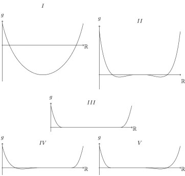
ξ hN
[image:16.595.160.480.109.256.2](b)
Figure 1.1: These are sketches of (a) the IRW(see (1.2)) and (b) the linear inter-polationhN (see (1.12)). Note that in (a) the jump heights correspond to (Yn)N∈N, the third jumpY3 is highlighted.
the linear interpolation of the scaled IRW N12ζ. So the scaling N12 we obtain an
LDPfor theIRWif we use the scaling N12. Note that the increments (Yi)i∈Nhave a variance of orderN and that hence theIRWshas a variance of orderN3. Hence the IRWscaled byN13/2 has a variance of order 1. In fact forJ =−∞theIRWscaled by
1
N3/2 converges to the integrated Brownian motion, in [11] Caravenna and Deuschel
use Donskers Invariance Principle to prove this. The integrated Brownian motion is a stochastic object and since we want to prove a principle of large deviations for
the empirical profile on (C,k·k∞) we use the scaling N12 instead of the scaling
1
N3/2.
We study the sequences
γaN :=Pψ◦h−N1,
γrN :=γrN,−∞:=γNψ,−∞◦h−N1,
ˆ
γrN :=γrN,J :=γNψ,J◦h−N1,
[image:16.595.250.392.489.543.2]where ψ = ψr,N. For an illustration of the IRW and its linear interpolation see Figure 1.1. We say that the interface (γNr)N∈N has left boundary valuea and right boundary valuebbecauseN−2ψr,N(0)≡aandN−2ψr,N(N)≡b; we say that it has left gradientα and right gradient β because
N−2ψr,N(0)−N−2ψr,N(−1)
N−1 ≡α and
N−2ψr,N(N+1)−N−2ψr,N(N)
N−1 ≡β.
Theorem 1.2. The sequences of measures(γN)N∈N= (γNa)N∈N,(γNr)N∈Nsatisfy in (C(0,1),|| · ||∞) the large deviation principles with speedN and good rate functions
Σa and Σr of the form
Σ(f) :=
Q(f)−Q(H) , forf ∈H,
∞ , otherwise.
(1.14)
Where Q : H2(0,1) → R is the functional on the Sobolev space H2 (the set of functions for which the second weak derivative is in L2) defined by
Q(f) := 1 2
Z 1
0
( ¨f(ξ))2dξ,
where for every subset A of H2 the expression Q(A) denotes the infimum of Q in A, and where H=Ha or Hr with
Ha:={f ∈H2 |f(0) =a,f˙(0) =α},
Hr:={f ∈H2 |f(0) =a,f˙(0) =α, f(1) =b,f˙(1) =β}. (1.15)
For the case without terminal condition we can go beyond the case where the random variable X1 from the random walk representation (1.2) has the standard normal distribution.
The central theorem of this thesis is the LDP for the model with pinning interaction, (γNr,J)N∈N. We will use theLDPfor the model without pinning to prove
the one for model with pinning. We will apply that theLDPfor the model without
pinning tells us that for a measurable subsetAinC(0,1) the probability ofAunder
γNr is for large N approximatelye−NΣr(A): Fix >0, by the LDPupper and lower bounds there is anN0 such that for N > N0 we have
e−N(Σr(Ao)+)≤γNr(A)≤e−N(Σr( ¯A)−), (1.16)
where ¯Ais the closure andAo is the interior of the setA. Note thatN0 depends on the set A and the boundary condition r. In our application of this approximation we have to take care of this dependence.
large deviation principle with speedN and rate function
Σr,J(f) :=
EJ(f)− EJ(H
r) , forf ∈Hr,
∞ , otherwise,
(1.17)
where EJ:H
r→R is given by
EJ(f) = 1
2
Z 1
0
( ¨f(ξ))2dξ−τ(J)|Nf|, (1.18)
where |Nf|is the Lebesgue measure of the zero set Nf :={ξ ∈[0,1]|f(ξ) = 0} and EJ(H
r) = inff∈HrE
J(f).
For the gradient model the LDPs for the corresponding models are known
(see [5], [19]). To obtain them the scaled fields (N1φξN)ξ∈ΛN/N are used and hence
hN(φ)(ξ) := N1φbN ξc+ (ξ− bN ξc
N )
1
N(φbN ξc+1−φbN ξc) , forξ∈[0,1].
The boundary condition for the gradient model is given by
ψ∇,r,N(i) :=
aN , fori= 0,
bN , fori=N,
0 , otherwise,
wherer= (a, b).
Funaki and Sakagawa [19] prove that the empirical profile of the gradient
model γN∇,J ◦(hN)−1 with boundary condition ψ = ψ∇,r,N satisfies an LDP in
(C(0,1),k·k∞) with speedN and rate function
Σ∇,J(f) :=
E∇,J(f)− E∇,J(H) , forf ∈H,
∞ , otherwise,
whereH contains all functions from the Sobolev spaceH1 that are equal toaat 0 and equal tobat 1, and where
E∇,J(f) = 1 2
Z 1
0
( ˙f(ξ))2dξ−τ(J)|Nf|.
with lag 1. These tools allow the authors of [19] to proof theLDPforJ >−∞with the help of theLDPforJ =−∞. Funaki and Sakagawa [19] use the random walk representation to prove the LDP for J = −∞ as follows: they use the Mogulskii
theorem (see Theorem A.3) to derive an LDP for the random walk Y and since
the processY is Gaussian the well known Gaussian bridge (see Appendix B) allows the authors of [19] to implement the condition thatY(N) =bN via the contraction principle.
To see the convenience of the splitting property with lag 1 for the proof of theLDPwithJ >−∞, consider the term in the expansion that corresponds to the setS = ΛN \ {p}: By the splitting property with lag 1 we have
eJZS∇,ψγS∇,ψ(A) =eJZ{∇1,ψ,2,...,p−1}γ{∇1,ψ,2,...,p−1}(A)Z{∇p,ψ+1,p+2,...,N}γ{∇p,ψ+1,p+2,...,N}(A).
The main reason why the authors of [19] can use the LDPfor J = −∞ to prove
the LDP for J > −∞ is that the Gibbs measure γ{∇1,ψ,2,...,p−1} where ψ = ψ∇,r,N
coincides with the Gibbs measure γΛ∇,ψ
p where ψ = ψ
∇,˜r,p and where ˜r = (aN p,0).
We can treatγ{∇p,ψ+1,p+2,...,N} analogously.
For the Laplacian model the measures only have a splitting property of lag
2 and hence using the LDP for J = −∞ to prove the LDP for J > −∞ is more
complex.
In terms of the LDP, the main difference between the gradient and the
Laplacian model is the smoothness of the minimisers of the rate functions: in the
Laplacian case they have to be continuously differentiable (and the second weak
derivative has to exists in L2) whilst in the gradient case they do not need to be continuously differentiable.
Note that Funaki and Otobe [18] study the LDP for the gradient model
under more general assumptions. For the models studied in [18] the random walk representation is not necessarily a Gaussian process. So the authors can not use
the Gaussian bridge in their proof of the LDP for J = −∞. Instead they use a change of measure approach. But to apply the change of measure the authors use that the gradient field satisfies a splitting property with lag 1. For a proof of the
LDPfor J > −∞ the authors of [18] refer the reader to the proof of Funaki and Sakagawa [19].
The minimiser of the rate function is not unique
the rate function Σr,J of the LDP. To see that the set M∗
r contributes to our
understanding of the behaviour of the interface model (ˆγNr)N∈Nfor large N letA⊂
C(0,1) be an open set that containsM∗
r. By theLDPwe have limN→∞γˆN(A) = 1.
So if the set M∗r coincides with the minimiser of the rate function Σr,−∞ of the
model without pinning, then the pinning reward J has no effect on behaviour of the empirical profile. We will see that for non zero boundary conditionr6= 0 there
is always a critical reward strictly larger then Jc (recall that Jc is the reward until
which the pinning free energy, with zero boundary conditions, is zero) such that for smaller rewards the pinning has no effect.
Furthermore, it turns out that there are boundary conditions such that the
minimiser is not unique. In the extreme case the set of minimisers contains five functions, one of them has a zero set of Lebesgue measure zero and the other ones
have a zero set of strictly positive Lebesgue measure. We present them in Section 4.
For the gradient case there are also boundary conditions such that the min-imiser is not unique. Here up to two minmin-imisers exist, one touching and one not
touching zero.
Fixing boundary conditions such that two minimisers exist and considering for each minimiser an arbitrarily small ball around it we study the probability to
observe an interface in one of these balls given that N is large. If for one ball the probability is arbitrarily close to one for large N, we say the empirical profile concentrates at the minimiser corresponding to this ball. For the gradient model
Bolthausen, Funaki and Otobe [5] study the concentration behaviour of the em-pirical profile. They show that the probability to observe an interface in the
neigh-bourhood of the minimiser that picks the reward is arbitrarily close to one while the
probability to observe one near to the minimiser that does not pick the reward is close to zero.
For the Laplacian model we outline an approach for discussing the
concen-tration in Chapter 5. We claim that concenconcen-tration behaviour of the Laplacian model is completely opposite to the behaviour of the Gradient model: the probability to
observe an interface in the neighbourhood of the minimiser that picks the reward
is arbitrarily small while the probability to observe one near to the minimiser that does not pick the reward is close to one.
Fluctuations
For zero boundary conditions, the LDP tells us that the empirical profile for the Laplacian model is close to the zero line with a probability close to one. In other
Caravenna and Deuschel [11] show that the typical height ofφi isN
3/2 forJ < J
c,
O((logN)2) for J > Jc and O(N 3/2
logN) for J = Jc (see [11, Theorem 1.2, Theorem
1.4]). In particular the authors of [11] show that the law of the linear interpolation
of N1s(φξN)ξ∈ΛN/Nwhere the scalingsis
3
2 converges forJ < Jcin distribution to the law of the integrated Brownian motion bridge and forJ ≥Jcto the law concentrated
on the constant functionf(ξ) = 0 (see [11, Theorem 1.2]).
Related models
Models that are related to the (1+1)-dimensional models, are the (d+1)-dimensional models. The elements of the state space of these models are given by
{φi}i∈Zd, whereφi∈R.
Using the d dimensional discrete gradient and Laplacian, we can define (d+ 1)-dimensional models.
In statistical physics a natural next step after defining a family of Gibbs distributions is to study the existence of a so calledGibbs measure(see [20, Definition
2.9]). A Gibbs measure is a measureγ of a random field on Zdthat satisfies for all
finite subsets Λ⊂Zd that
γ(· | FΛc)[ψ] =γψ
Λ γ-a.s.,
whereFΛc is theσ-algebra generated by{φj |j6∈Λ}. For the gradient model such
a Gibbs measure exists if and only ifd≥3 (see [20, Example 13.9]) whilst for the Laplacian model such a Gibbs measure exists if and only ifd≥5 (see [27] or [25]). So for the gradient model the dimension d = 2 and for the Laplacian model the dimensiond= 4 are the critical dimensions after which a Gibbs measure exists.
For (d+ 1)-dimensional models, localisation and delocalisation have been studied: for the gradient model we haveJc=−∞for all d≥1, see [29, Section 5],
and for the Laplacian model it is shown in [28, Theorem 1] thatJc=−∞ford≥4.
An interesting phenomenon that has been studied for (d+ 1)-dimensional models isentropic repulsion. In statistical physics entropic repulsion referrers to the behaviour of an interface near to a wall (see [7]). An interface shows this behaviour
if the interface is flat in the absence of a wall but divergent in the presence of a wall.
Intuitively we explain this phenomenon by the fact that the interface that diverges from the wall has more space for fluctuation compared to the one that stays close to
the wall. Mathematically, the wall is modelled by conditioning the Gibbs measure
For the gradient model entropic repulsion has been studied in [4] for
dimen-sionsd≥3. Bolthausen and Deuschel [4] show that there is a constantC such that the interface (φi)i∈ΛN has a height of approximately
√
ClogN. In [4] the constant
C is given explicitly. For the critical dimension d = 3 Bolthausen, Deuschel and Giacomin [3] prove that there is a constantC such that the maximum of the Gibbs distribution is pushed to the height ClogN.
For the Laplace model, the first rigorous results concerning entropic repulsion
are in [27]. Sakagawa [27] proves lower and upper bounds for the probability to have positive heights. Kurt [25] proves an upper bound that asymptotically matches the
lower bound of [27]. The author of [25] deduces that as for the gradient model
there is a constant C such that for d ≥ 5 the heights of the Laplacian model are approximately repelled to a level of√ClogN. Furthermore Kurt [26] considers the critical dimensiond= 4: The local sample mean of the field is pushed to ClogN, whereC is some constant.
A different generalisation are the (1 +s)-dimensional models. The elements of the state space are given by
{φi}i∈Z, whereφi ∈Rs.
For the gradient model, localisation and delocalisation is studied in [5, Theorem
1.1].
A further direction of generalisation is to allow other interactions. For
ex-ample Borecki [6] studies localisation and delocalisation for models with the
Hamil-tonian
H(φ) =X
i
(κ1(∇φi)2+κ2(∆φi)2),
where κ1 and κ2 are positive constants. The main observation for this (∇+ ∆) model is that forκ1 >0 the model is localised for allJ >−∞, independently of the parameterκ2. So ifκ1 >0 the localisation behaviour of the (∇+ ∆) model is the same as the one of the pure gradient model. The Laplacian interaction influences
the (∇+ ∆) model only if κ1 = 0.
A further model that is related to the model with pinning interaction is
the model with wetting interaction. The model with wetting interaction differs
from the model with pinning interaction by the way the polymer interacts with the environment. Mathematically, the model with wetting interaction and the model
with pinning interaction differ by the definition of the reference measure. We obtain
stay in the positive half plane. Hence for models with wetting we should observe a
competition between the effects of entropic repulsion and pinning. For the Laplacian model this was studied in [10] for d= 1. Caravenna and Deuschel [10] prove that the critical reward for the model with wetting interaction is strictly larger than the
critical reward for the model with pinning interaction. Furthermore they show that the transition from delocalised to localised behaviour is of first order or in other
words that the first derivative of the free energy of the model for wetting has a
discontinuity, see [10, Theorem 1.3].
Overview
In Chapter 2 we prove theLDPsfor the models without pinning, see Theorem 1.2.
For the proof of the LDP for the model without terminal boundary conditions,
(γNa)N∈N, we use that, by the random walk representation (1.2), the the gradient of
this field is a random walk with i.i.d. increments. We apply Mogulskii’s theorem to get anLDPfor this random walk. Then we use the contraction principle to extend
theLDPfor the random walk to anLDPfor the integrated random walk.
The second model that we consider in Chapter 2 is the Laplacian model without pinning and with boundary condition zero on both sides. To obtain an
LDP for this model we use the Gaussian bridge. We will see that the Gaussian
bridge corresponds to a contraction map. In a last step we extend the LDP for zero boundary conditions to the LDP for non zero boundary condition. For this
extension we show that for each non zero boundary condition there is a sequence of
image measures of the measure with zero boundary conditions that is exponentially equivalent to the sequence with non zero boundary condition.
Funaki and Sakagawa [19] use this procedure to derive anLDPfor the model
with terminal boundary condition for the gradient model. But since the random walk representation of the gradient model without terminal boundary conditions
is a random walk with i.i.d. increments, the LDP of the gradient model without
terminal boundary conditions follows directly via Mogulskii’s theorem. Furthermore the gradient model with terminal boundary conditions is only conditioned on one
boundary point namely N while the Laplacian model is conditioned at two points namely atN and N+ 1. So the Gaussian bridge for the Laplacian model depends on φ(N) and φ(N + 1), whilst the one for the gradient model does not depend on
φ(N+ 1).
probabil-ities of certain subsets ofC(0,1) (like the upper bound from (1.16)) hold uniformly for a certain family of intervals and boundary conditions.
In Chapter 3 we prove theLDPfor the Laplacian model with pinning
inter-action, see Theorem 1.3. Therefore we use the two stage interpretation (1.6). For
the gradient model, Funaki and Sakagawa [19] also use a two stage interpretation of the pinned measure. Since the gradient model satisfies the splitting property with
lag 1, the authors of [19] can use theLDP for the model without pinning to prove
the LDPfor the model with pinning. For the Laplace model this property is not satisfied. Especially for the upper bound this forces us to use more complex
meth-ods than the authors of [19] did. In order to use the LDP for the model without
pinning we apply a generalisation of the law of total expectation.
In Chapter 4 we study the minimisers of the rate function. For certain
bound-ary conditions and rewards the minimiser is not unique and the set of minimisers
contains up to five different minimisers.
In Chapter 5 we give an outlook and a conclusion. We present a
possi-ble approach for dealing with the concentration propossi-blem and describe some of the
problems related to the wetting model.
We provide four appendices. In Appendix A we collect the results from
large deviation theory that we apply in this thesis. Then, in Appendix B, we give some well known facts about finite dimensional Gaussian measures. Furthermore,
in Appendix C, we analyse the partition function for the model without pinning.
Chapter 2
Integrated random walk
In this chapter we prove Theorem 1.2. In Section 2.1 we consider the empirical profiles of the models without terminal condition, (γa
N)N∈N. In Section 2.2 we
consider the integrated random walk conditioned to have zero boundary conditions
on both sides. In Section 2.3 we extend the LDP from Section 2.2 to models
with none zero boundary condition. For this extension we use that the bridge of a
Gaussian random walk is well known (see Appendix B). In our proof of Theorem 1.3
we use certain extensions of the Theorem 1.2, we present them in Section 2.4. The approach to prove theLDPfor the model with boundary conditions on
both sides by first proving the one for the model with boundary conditions on only
one side and then using the Gaussian bridge has been used already for the gradient model in [19]. In [12] the same procedure has been suggested for the Laplacian case.
2.1
Integrated random walk sample path large
devia-tions
In this section we prove Theorem 1.2 for the models without terminal condition.
Therefore we use the random walk representation (1.2). We study the empirical profile hN(ζ) of the IRW ζ. Our proof works under a more general assumption
thanX1 being Gaussian: It is enough if the log moment generating function Λ(λ) := logE[eλX1] is finite for allλ∈RandE[X1] = 0. We prove anLDPfor the empirical
profile of the IRWor in other words for ϑa
N := Pψ ◦h
−1
N where ψ=ψr,N (for the
definition ofψr,N see (1.13)) andPψ is such thatX1 has a finite moment generating function.
large deviation principle with speedN and good rate function
Πa(f) :=
R1
0 Λ
∗( ¨f(ξ)) dξ−inf
g∈H˜a
R1
0 Λ
∗(¨g(ξ)) dξ , forf ∈H˜ a
∞ , otherwise,
(2.1)
where H˜a are the functions f such that the first derivative is absolutely continu-ous and such that f(0) = a and f˙(0) = α, and where Λ∗ is the Fenchel-Legendre transform ofΛ:
Λ∗(ξ) := sup
λ∈R
[λξ−Λ(λ)].
Proof. First we prove the proposition for a = 0 and then we extend the proof to
the casesa∈R2. Finally we show the goodness of the rate function Πa.
Case a = 0: For this case we use a small extension of Mogulskii’s Theorem (see
Theorem A.3) and thecontraction principle (CP)(see Theorem A.4). Therefore
note thathN(ζ) is the image ofξ 7→N−1YbN ξc+1 under the integral operator:
hN(ζ)(ξ) = N12ζbN ξc+ N12 Z ξ
bN ξc
N
(ζbN sc+1−ζbN sc) ds= N1
Z ξ
0
YbN sc+1ds. (2.2)
The integral operator is a continuous map from (L∞(0,1),k·k∞) to (C(0,1),k·k∞)
because it is linear and bounded. Additionally, by Proposition 2.2 below the
se-quence of laws of (ξ 7→N−1YbN ξc+1)N∈N satisfies anLDPin (L
∞(0,1),k·k
∞) with
rate functionIM, where
IM(f) :=
R1
0 Λ
∗( ˙f(ξ)) dξ , forf ∈ AC, f(0) = 0,
∞ , otherwise,
(2.3)
and whereACare the absolutely continuous functions. So, by theCP, the sequence (ϑN)N∈N satisfies anLDPwith rate function
f 7→ inf
g∈Sf
IM(g) , whereSf ={g∈L∞(0,1)|Rξ
0g(s) ds=f(ξ) , forξ ∈[0,1]}. (2.4)
By considering two cases we see that the functions (2.4) and Π0are equal. Iff(0)6= 0 or iff is not differentiable, then we have Sf =∅; because the image of the integral
Case a ∈R2: For non zero boundary conditions we use that the IRWwith zero
boundary conditions and the one for the boundary conditionψr,N differ by the linear trend i7→ aN2+iN α. Hence for N → ∞, the empirical profiles differ by a+ξα. This two observations allow us to prove the proposition by applying the exponential
equivalence and theCP. Therefore we use the operatorsKf:C(0,1)→C(0,1) and
Kϕ:RΛN →RΛN given by
Kf(h)(ξ) =h(ξ)−f(ξ) , for allξ∈[0,1]. (2.5)
and
Kϕ(φ)i =φi−ϕi. (2.6)
We show that (ϑaN)N∈Nand (ϑ0N◦Kha)N∈N, whereha(ξ) =a+ξα, are exponentially equivalent. Note
ϑaN =Pψ◦hN−1 =P0◦Kφa,N ◦h −1
N ,
whereφa,N(i) =aN2+iN α. The sequence (P0◦Kφa,N ◦h −1
N )N∈N is exponentially equivalent with the sequence (P0◦h−N1◦Kha)N∈N, because
lim
N→∞kKφa,N ◦(hN)
−1(f)−(h
N)−1◦Kha(f)k∞= 0 for all f ∈C(0,1),
where the norm k·k∞ is the uniform norm on RΛN (see Example A.6). Since we
haveP0◦h−N1◦Kha =ϑ0N ◦Kha and since (ϑ0N◦Kha)N∈Nhas, by theCP, the rate Πa the exponential equivalence shows that (ϑaN)N∈N also has the rate Πa.
Goodness of the rate function: The rate function Πa is good because the rate
function IM is good and because goodness is preserved under the CP. (For the Gaussian case we present an alternative proof of the goodness in Section 2.4.1).
Proof of Theorem 1.2 for models without terminal condition. Since for the normal distribution we have Λ∗(x) = 12x2, Proposition 2.1 implies that Theorem 1.2 is true for (γNa)N∈N.
The following proposition is a small adaptation of Mogulskii’s theorem (see
Theorem A.3).
Proposition 2.2. Under P0, the sequence of laws of(ξ7→N−1YbN ξc+1)N∈N satis-fies anLDPon(L∞(0,1),k·k∞) with rate functionIM; whereIM is given in (2.3) above.
Proof. Recall that by Mogulskii’s theorem (see Theorem A.3), the sequence of laws
of (ξ7→N−1YbN ξc)N∈Nsatisfies in (L
∞(0,1),k·k
the rate function IM. We prove that IM is also the rate function for the sequence of laws of (ξ7→N−1YbN ξc+1)N∈N, by proving that (ξ7→N
−1Yb
N ξc+1)N∈Nand (ξ7→
N−1Y
bN ξc)N∈Nare exponential equivalent (see Definition A.5 and Theorem A.7).
For all ξ ≤ 1, the difference |N−1YbN ξc+1 −N−1YbN ξc| = |N−1XbN ξc+1| is bounded from above by the maximumN−1maxi≤N+1|Xi|, and hence for anyη >0,
we have
P0(kN−1YbN ξc+1−N−1YbN ξck∞> η)≤P0(N−1 max
i≤N+1|Xi|> η).
Exponential equivalence follows by Proposition 2.3 below.
We frequently use the following result to prove exponential equivalence.
Proposition 2.3. For all η >0,
lim sup
N→∞
1
N logP
ψ( max
i≤N+1|Xi|> ηN) =−∞.
Proof. Since the distribution of the random variableX1is not effected by the bound-ary condition, we use the notation P = Pψ in this proof. For every λ > 0, by exponential Chebyshev’s inequality,
P( max
i≤N+1|Xi|> ηN)≤(N + 1)P(|X1|> ηN)≤(N+ 1)E[e
λ|X1|]e−λN η.
Hence,
lim sup
N→∞
1
N logP(maxi≤N|Xi|> ηN)≤lim sup N→0
1
N log((N + 1)E[e
λ|X1|]e−λN η)
≤ −λη,
where we usedE[eλ|X1|]<∞ for all λ. Letλ→ ∞to finish the proof.
2.2
Integrated random walk bridge sample path large
deviations, with zero boundary condition
In this and the following section we prove Theorem 1.2 for γr
N. In this section we
assumer=0 and writeP :=P0.
Essential to our proof is that for the Gaussian measure P we can calculate explicitly a mapBN such thatPN =P◦B−N1 (see Section B). Note that for general
distributions other methods to obtain BN are necessary and hence we also need
We use the maps (BN)N∈N to show that there is a continuous map B such that
(P◦˜h−N1◦B−1)
N∈Nand (γN0)N∈N= (P◦B−N1◦h−N1)N∈N
are exponentially equivalent, where ˜hN :RN→C(0,1)×R is given by
˜
hN(ζ) := (hN(ζ),
1
N(ζ(N+ 1)−ζ(N)). (2.7)
We present such a mapB in the next proposition.
Proposition 2.4. Let L˜ :=C(0,1)×R with the norm k(f, v)k=kfk∞+|v|. The sequences (γN)N∈N and ( ˜ϑN)N∈N are exponentially equivalent, where
˜
ϑN :=P ◦h˜−N1◦B−1,
and
1. ˜hN is given in (2.7),
2. B: ˜L→C(0,1) is the continuous map given by
B(f, v)(ξ) =f(ξ)− A(ξ, f(1), v), where A:R3 →R is given by
A(ξ, u, v) = (3u−v)ξ2+ (−2u+v)ξ3.
We prove Proposition 2.4 below.
Proof of Theorem 1.2 forγr
N withr=0. By Proposition 2.4 it is enough to prove
that ( ˜ϑN)N∈N has the rate Σ0. Since B is continuous we first obtain an LDP for (P◦˜h−N1)N∈N in ˜Land apply theCP in a second step.
Step 1: We show that (P ◦h˜−N1)N∈N satisfies anLDPin ˜L with rate function
˜
Σ(f, v) =
1 2
R1
0( ¨f(ξ))2dξ , forf ∈H(0,0),f˙(1) =v,
∞ , otherwise.
(2.8)
We use the CP to prove (2.8) because P ◦˜h−N1 coincides with the law of ξ 7→
Φ(N−1Y
bN ξc+1) where
Φ(f) := ((
Z ξ
0
to verify this recall (2.2). Note that the linear map Φ : L∞ → L˜ is continuous because it is bounded due to
kΦ(f)k ≤ kfk∞+|f(1)| ≤2kfk∞.
So, by theCP and since IM(g) = ∞ ifg 6∈ AC, the rate function of (P ◦˜h−N1)N∈N is given by (f, v)7→infg∈S(f,v)IM(g), where
S(f,v):={g∈ AC |
Z t
0
g(ξ) dξ=f(t) for all t∈[0,1], g(1) =v}.
Since we haveS(f,v)6=∅only if there is a g∈ AC such that ˙f =g and hence such that in particular ˙f(1) =g(1) =v, we have
S(f,v)=
{f˙} , for ˙f ∈ AC, f(0) = 0,f˙(1) =v,
∅ , otherwise.
(2.9)
Since for the normal distribution we have Λ∗(x) = 12x2 and IM( ˙f) =∞ if ˙f(0)6= 0 the maps (2.8) and (f, v)7→infg∈S(f,v)IM(g) coincide.
Step 2: Now we use (2.8) to show that the rate function of ( ˜ϑN)N∈Ncoincides with
Σ0. SinceB is continuous theCP yields that the rate function of ( ˜ϑN)N∈Nis given byf 7→inf(g,v)∈Sf Σ(˜ g, v), where
Sf ={(g, v)∈L˜ |B(g, v) =f}.
Since ˜Σ(g, v) =∞ ifg6∈H(0,0) or if ˙g(1)6=v, we have
inf (g,v)∈Sf
˜
Σ(g, v) = inf
g∈S˜f
˜
Σ(g,g˙(1)),
where
˜
Sf :={g∈H(0,0)|B(g,g˙(1)) =f}. We show
˜
Sf =
{f +A(·, u, v)|(u, v)∈R2} , forf ∈H(0,0,0,0),
∅ , otherwise.
(2.10)
(H(0,0), <·,·>) toH(0,0,0,0), where<·,·>is the semi-inner-product given by
< f, g >:=
Z 1
0 ¨
f(ξ)¨g(ξ) dξ.
To check this note that the range of the map is actuallyH(0,0,0,0)and that, by Propo-sition D.1, the difference f −B(f,f˙(1)) = A(·, f(1),f˙(1)) minimisesf 7→< f, f >
inH(0,0,f(1),f˙(1)).
Now we use this property ofB to show that (2.10) is true. We first consider the case that f is not an element of H(0,0,0,0). Since the image of H(0,0) under B is H(0,0,0,0), the equation B(g,g˙(1)) = f has no solution g in H(0,0) if f is not an element of H(0,0,0,0), and hence for those f we have ˜Sf =∅. This implies that the
left and right hand side of (2.10) coincide in the case that f is not an element of
H(0,0,0,0). Now we consider the casef ∈H(0,0,0,0). Since the kernel of the orthogonal projection g 7→ B(g,g˙(1)) is {A(·, u, v)|(u, v)∈R2}, the left and right hand side
of (2.10) also coincide iff is an element ofH(0,0,0,0). Forf ∈H(0,0,0,0) we actually have
inf
g∈S˜f
˜
Σ(g,g˙(1)) = 12
Z 1
0
( ¨f(ξ))2dξ. (2.11)
To check (2.11) fixg∈S˜f and note that by (2.10) there is a vector (u, v)∈R2 such
thatg(ξ) =f(ξ) +A(ξ, u, v) and hence
˜
Σ(g,g˙(1)) = 12
Z 1
0
( ¨f(ξ))2dξ+
Z 1
0 ¨
f(ξ) ¨A(ξ, u, v) dξ+12
Z 1
0
( ¨A(ξ))2dξ.
By Proposition D.1 the minimiserA(·, u, v) is a polynomial of degree 3 and hence
Z 1 0
¨
f(ξ) ¨A(ξ, u, v) dξ= 0 , forf ∈H(0,0,0,0).
Furthermore,
Z 1
0
( ¨A(ξ, u, v))2dξ≥0
for all (u, v)∈R2 with equality if and only if (u, v) = (0,0). Combining these three facts we see that (2.11) is true.
Proof of Proposition 2.4. Step 1:
We show that there is a mapBN such that
Therefore we use the well known formula for Gaussian bridges (see [13] and
Ap-pendix B). For this purpose the alternative definition ofPN given by
PN(·) =P(·|ζN = 0,ζN+1−ζN = 0) (2.13)
is more convenient becauseζN+1−ζN =YN+1. By (B.1), we have
BN(ζ)(i) =ζi−
h
Ci,N Ci,N+1
i "
CN,N CN,N+1
CN,N+1 CN+1,N+1
#−1"
ζN
ζN+1−ζN
#
, fori≤N,
where Ci,N = E[ζiζN], Ci,N+1 = E[ζi(ζN+1 −ζN)] for all i ∈ {1,2, . . . , N} and
CN+1,N+1 =E[(ζN+1−ζN)2] = (N + 1) (where the expectations are with respect
toP). Since
Ci,N =E[ζiζN] =
1 6(−i
3+ 3N i2+i(3N + 1)) , fori≤N
andCi,N+1 =E[YN+1
Pi
x=1Yx] = 12i(i+ 1) fori≤N, we have
BN(ζ)(x) =ζ(x)−AN(x,ζ(N),ζ(N + 1)−ζ(N)), for allx∈ {1,2, . . . , N, N + 1},
(2.14)
whereAN: {1,2, . . . , N, N+ 1} ×R×R→Ris given by
AN(x, U, V) :=
1
N(N + 1)(N + 2)
x3[−2U +N V] +x2[3U N +V N −V N2]
+x[(2 + 3N)U−N2V] . (2.15)
Step 2By (2.12), the sequences (γN)N∈N and ( ˜ϑN)N∈N are exponential equivalent,
if underP for any η >0 the probability that
B(˜hN(ζ))(ξ)−hN(BN(ζ))(ξ) (2.16)
has a k·k∞-norm larger than η decays with an logarithmic rate of −∞. Let uN =
N−2ζ(N) and vN =N−1(ζ(N+ 1)−ζ(N)). By definition, (2.16) is equal to
hN[AN(i,ζ(N),ζ(N+ 1)−ζ(N))]− A
ξ,ζN(N2),
ζ(N+1)−ζ(N)
N
=
h
1
N2AN(ξN,ζ(N),ζ(N+ 1)−ζ(N)v)− A
ξ,ζN(N2),
ζ(N+1)−ζ(N)
N
i
+hN[AN(i,ζ(N),ζ(N + 1)−ζ(N))]−N12AN(ξN,ζ(N),ζ(N + 1)−ζ(N))
.
Hence, by applying Proposition 2.5 below to the first term on the right hand side
of (2.17) and by applying the definition ofhN to the second term on the right hand
side of (2.17), we see that (2.16) is
O(N1) max|ζN(N2)|,|
ζ(N+1)−ζ(N)
N |
, forN → ∞.
Since ζ(N) ≤ N2maxi≤N|Xi| and ζ(N + 1)−ζ(N) ≤ Nmaxi≤N+1|Xi|, (2.16) is
O(N1) maxi≤N+1|Xi|and hence there is aC such that
P(k(B(˜hN(ζ)))(ξ)−hN(BN(ζ))(ξ)k∞> η)≤P(CN−1 max
i≤N+1|Xi|> η).
Now the exponential equivalence follows by Proposition 2.3.
Proposition 2.5. For (u, v)∈R2 and ξ ∈[0,1]
|N12AN(ξN, N2u, N v)− A(ξ, u, v)|=O(N1) max (|u|,|v|). (2.18)
Proof. We consider the coefficients of the polynomial ξ 7→ N−2AN(ξN, N2u, N v):
By definition ofAN,
the coefficient of the leading term is
N3[−2uN2+vN2]
N3(N+ 1)(N + 2) = [−2u+v]
N2
(N+ 1)(N+ 2)
= (−2u+v) +O(N1) max(|u|,|v|) , forN → ∞, (2.19)
the second order term is
N2[3uN3+vN2−vN3]
N3(N+ 1)(N+ 2) = [3u−v+
v N]
N2
(N + 1)(N + 2)
= (3u−v) +O(N1) max(|u|,|v|) , forN → ∞,
(2.20)
the first order term is
N[2uN2+ 3uN3−vN3]
N3(N + 1)(N + 2) =O( 1
N) max(|u|,|v|) , forN → ∞, (2.21)
and the constant term is zero.
Combining the definition of A with (2.19), (2.20) and (2.21), we see that (2.18) is
2.3
Integrated random walk bridge sample path large
deviations, non zero boundary condition
In this section we give the remainder of the proof of Theorem 1.2. We extend the part of Theorem 1.2 that we already proved to the case where the boundary conditions
are not zero. In the following we provide the central tool for this extension.
Lemma 2.6. The sequences(γNr)N∈N and(γN0 ◦Khr)N∈N are exponentially
equiva-lent inC(0,1), wherehr is the unique minimiser of Qin the set Hr, and where the operatorKf:C(0,1)→C(0,1)is given in (2.5).
Proof. Central to our proof is that γr
N and γN0 ◦Khr are image measures ofγ
0
N: In
fact, as we will show at the end of this proof, we have
(γNr )N∈N= (γ
0
N◦Kφr◦(hN)
−1)
N∈N
(γN0 ◦Khr)N∈N= (γ
0
N◦(hN)−1◦Khr)N∈N, (2.22)
where φr is the minimiser of HN in the set that satisfies the boundary condition
ψ = ψr,N (see Proposition D.2, note that we drop the index N here and write
φr,N =φr) and whereKϕ:RΛN →RΛN is given in (2.6).
Exponential equivalence follows from (2.22) because, by Proposition D.2, the
sequence (hN(φr))N∈N converges tohr and hence
lim
N→∞kKφr◦(hN)
−1(f)−(h
N)−1◦Khr(f)k∞= 0 for all f ∈C, (2.23)
where the normk·k∞ is the uniform norm onRΛN.
Statement (2.23) shows that (2.22) is sufficient to prove the exponential
equivalence, now we show that (2.22) is actually satisfied. Therefore note that by the definition ofγN0 the image measure γN0 ◦Khr has the claimed form. It remains to show that
γNψ =γN0 ◦Kφr, forψ=ψ
r,N. (2.24)
Proposi-tion D.2): In the first place it implies that
ZNψ =
Z
RΛN
e− HN(φ) Y
i∈ΛN
(dφi)
Y
i∈{−1,0,N,N+1}
δψi(dφi)
=
Z
RΛN
e− HN(φ−φr)−HN(φr) Y
i∈ΛN
dφi
Y
i∈{−1,0,N,N+1}
δψi(dφi)
=e− HN(φr)
Z
RΛN
e− HN( ˜φ) Y
i∈ΛN
(d ˜φi)
Y
i∈{−1,0,N,N+1}
δ0(d ˜φi)
=e− HN(φr)Z0
N, (2.25)
where in the third line we substitutedφ−φr =Kφr(φ) by ˜φ; and in the same fashion the orthogonality property implies that
γNψ(A)
= 1
ZNψ
Z
A
e− HN(φ) Y
i∈ΛN
(dφi)
Y
i∈{−1,0,N,N+1}
δψi(dφi)
= e
HN(φr)
Z0
N
Z
A
e− HN(φ−φr)−HN(φr) Y
i∈ΛN
dφi
Y
i∈{−1,0,N,N+1}
δψi(dφi)
= 1
Z0
N
Z
Kφr(A)
e− HN(φ) Y
i∈ΛN
(dφi)
Y
i∈{−1,0,N,N+1}
δ0(dφi)
=γN0 ◦Kφr(A),
for any measurable setA.
Proof of Theorem 1.2. By Lemma 2.6 and the CP the rate function of the model
withJ =−∞ and boundary conditionris given by
f 7→Σ0(K−hr1(f)) = Σ0(f −hr).
This rate function is only finite iff−hr∈H0or in other words iff ∈Hr. Forf ∈Hr
we have by definition of Σ0 that Σ0(f−hr) =Q(f−hr). By the orthogonality ofhr
(see Proposition D.1) we see that this rate function and the one from Theorem 1.2
2.4
Preparation for the proof of Theorem 1.3
In this section we present results that we use in our proof of Theorem 1.3. In
Section 2.4.1, we prove the goodness of the rate functions Σa and Σr. In our proof of Theorem 1.3, we use the expansion (1.6). Therefore we need upper and lower
bounds toγSψ(Q) where S is of the formS ={s∗+ 1, s∗+ 2, . . . , s∗−1}=: (s∗, s∗) for s∗, s∗ ∈ N. In Section 2.4.2, we extend the LDP from Theorem 1.2 such that
we can apply it to the measures γSψ. Finally we show an uniformity result for the upper bounds derived from this extension of theLDP, see Section 2.4.3.
2.4.1 Goodness of the rate function
We prove that Σa and Σr are good rate functions. Note that this follows already
from the fact that the contraction principle preserves the goodness of the rate
func-tion. The main reason for presenting the proof as follows is that we use the same techniques to prove the goodness of Σr,J forJ >−∞.
To show that Σaand Σrare good rate function we have to show (by definition
of goodness) that they are lower semicontinuous function with compact level sets. By the definitions of Σa and Σr (see Theorem 1.2) it is sufficient to show that Q
has compact level sets (Lκ)κ∈R in (C(0,1),k·k∞), where
Lκ:={f ∈Ha|Q(f)≤κ}.
We start by showing that the sets (Lκ)κ∈R are closed.
Lemma 2.7. The level sets (Lκ)κ∈R are closed in (C(0,1),k·k∞).
Proof. Fix a level set Lκ and let (hn)n∈N be a uniformly converging sequence in Lκ with limit h ∈ C(0,1). We prove that h ∈ Lκ. The sequence (k¨hnk2L2)n∈N is bounded by 2κ because (hn)n∈N⊂Lκ andQ(hn) =
1
2kh¨nk2L2. SinceL2 is a reflexive
space there is a subsequence such that (¨hnk)k∈Nconverges weakly inL
2 to a function
g. By weak convergence we have
kgkL2 ≤lim infk¨hnkkL2. (2.26)
We showg= ¨h: Since the boundedness of (k¨hnkL2)n∈
N implies by
[ ˙hn(ξ)−h˙n(0)]2= [
Z ξ
0 ¨
hn(s)ds]2 ≤ kh¨nk2L2
sequence ( ˙hnk0)k0∈Nconverging to a function ˜g. By definition of the weak derivative we have
Z
˙
hnk0(ξ)f(ξ) dξ=−
Z
hnk0(ξ) ˙f(ξ) dξ , for all f ∈C
1
0. (2.27)
Taking the limitk0 → ∞ on both sides of (2.27), yields
Z
˜
g(ξ)f(ξ) dξ=−
Z
h(ξ) ˙f(ξ) dξ , for all f ∈C01,
where we used that inL2 the sequence (h
nk0)k0∈N converges toh (since it does so in
L∞) and ( ˙hnk0)k0∈N converges to ˜g. So ˙h = ˜g. Repeating this for ¨hnk we getg= ¨h.
Hence by (2.26)
kh¨kL2 ≤lim infkh¨nkkL2. (2.28)
Applying the definition ofQto (2.28) yields
Q(h)≤lim infQ(hnk).
Soh∈Lκ; and as h was arbitrary this implies thatLκ is closed.
Now we show thatLκ is compact.
Lemma 2.8. The level sets (Lκ)κ∈R are compact.
Proof. By Lemma 2.7 the level set Lκ is closed; so it suffice to show that Lκ is
precompact. By Arzel`a-Ascoli,Lκis precompact if it is bounded and equicontinuous.
Boundedness follows after two application of the fundamental theorem of calculus: Note, for all f ∈ Lκ, the norm kf¨kL2 is bounded. Since ˙f(x) = ˙f(0) + Rx
0 f¨(ξ) dξ, the boundedness ofkf˙k∞is a consequence of Jensen’s inequality applied toR0xf¨dξ: |Rx
0 f¨dξ| ≤ kf¨kL2. Sincef(x) =f(0) + Rx
0 f˙, the norm kfk∞is bounded as well.
To prove equicontinuity we have to show that for each >0 there is a δ >0 such that for allf ∈Lκ
if |y−x|< δ, then |f(y)−f(x)|< . (2.29)
From the proof of boundedness, we knowkf˙k∞ is bounded by a constantC; so we
have
f(y)−f(x) =|
Z y
x
˙
Hence, for all >0 and forδ= C, the inequality (2.29) is satisfied for allf ∈Lκ.
2.4.2 Extension of Theorem 1.2
In our proof of Theorem 1.3, we use the expansion (1.6). Therefore we need upper and lower bounds toγSψ(Q) whereS is of the formS ={s∗+ 1, s∗+ 2, . . . , s∗−1}=: (s∗, s∗) fors∗, s∗ ∈N. Motivated by the observation that a sample fromγψS◦h−N1 is fixed outside ofI = (s∗/N,s∗/N), we prove anLDPfor
γN,Ir :=γIψ N ◦
˜
h−N1, forψ=ψr,N,I, (2.30)
whereI is an interval in [0,1] with rational end pointsI∗< I∗, whereIN :=IN∩Z,
where ˜hN(φ) is the restriction ofhN(φ) toI and where
ψir,N,I :=
aN2−αN , fori=bN I∗c −1,
aN2 , fori=bN I∗c,
bN2 , fori=dN I∗e,
bN2+βN , fori=dN I∗e+ 1,
0 , otherwise,
and where forx∈Rthe value dxe is the smallest integer larger than or equal to x.
Note that the image of the interpolation ˜hN is the space of continuous
func-tions onI, we denote this space by C(I). We frequently use the following notation: ForQ ⊂C(0,1), the measureγN,Ir (Q) is the measure of the set of restrictions of the functions inQ to functions in C(I).
Proposition 2.9. The sequence of measures (γN,Ir )N∈N satisfies a large deviation
principle in the space (C(I),k·k∞) with speed N and good rate function ΣrI that is given by
ΣrI(f) =
QI(f)−QI(Hr(I)) , for f ∈Hr(I),
∞ , otherwise,
(2.31)
where
QI(h) = 12
Z
I
(¨h(ξ))2dξ. (2.32)
and