warwick.ac.uk/lib-publications
Original citation:Balogh, J, Hu, P, Lidicky, B, Pikhurko, Oleg, Udvari, B and Volec, Jan. (2015) Minimum number of monotone subsequences of length 4 in permutations. Combinatorics, Probability and Computing, 24 (4). pp. 658-679.
Permanent WRAP URL:
http://wrap.warwick.ac.uk/79457
Copyright and reuse:
The Warwick Research Archive Portal (WRAP) makes this work by researchers of the University of Warwick available open access under the following conditions. Copyright © and all moral rights to the version of the paper presented here belong to the individual author(s) and/or other copyright owners. To the extent reasonable and practicable the material made available in WRAP has been checked for eligibility before being made available.
Copies of full items can be used for personal research or study, educational, or not-for profit purposes without prior permission or charge. Provided that the authors, title and full bibliographic details are credited, a hyperlink and/or URL is given for the original metadata page and the content is not changed in any way.
Publisher’s statement:
© Cambridge University Press.
http://dx.doi.org/10.1017/S0963548314000820
A note on versions:
The version presented here may differ from the published version or, version of record, if you wish to cite this item you are advised to consult the publisher’s version. Please see the ‘permanent WRAP url’ above for details on accessing the published version and note that access may require a subscription
Minimum number of monotone subsequences of length 4
in permutations
J´ozsef Balogh
∗Ping Hu
†Bernard Lidick´
y
‡Oleg Pikhurko
§Bal´azs Udvari
¶Jan Volec
kNovember 13, 2014
Abstract
We show that for every sufficiently large n, the number of monotone subsequences of length four in a permutation onnpoints is at least bn/43c+ b(n+1)4 /3c+ b(n+2)4 /3c. Furthermore, we characterize all permutations on [n] that attain this lower bound. The proof uses the flag algebra framework together with some additional stability ar-guments. This problem is equivalent to some specific type of edge colorings of complete graphs with two colors, where the number of monochromatic K4’s is minimized. We
show that all the extremal colorings must contain monochromatic K4’s only in one of
the two colors. This translates back to permutations, where all the monotone subse-quences of length four are all either increasing, or decreasing only.
Keywords: flag algebras, permutation, pattern, density
∗Department of Mathematics, University of Illinois, Urbana, IL 61801, USA and Bolyai Institute,
Univer-sity of Szeged, Szeged, [email protected]. Research is partially supported by Simons Fellow-ship, NSF CAREER Grant DMS-0745185, Arnold O. Beckman Research Award (UIUC Campus Research Board 13039) and Marie Curie FP7-PEOPLE-2012-IIF 327763.
†Department of Mathematics, University of Illinois, Urbana, IL 61801, USA,[email protected]. ‡Department of Mathematics, University of Illinois, Urbana, IL 61801, USA,[email protected]and
Charles University in Prague. Research is partially supported by NSF grant DMS-1266016.
§Mathematics Institute and DIMAP, University of Warwick, Coventry CV4 7AL, UK,
[email protected]. Research is partially supported by ERC grant 306493 and EPSRC
grant EP/K012045/1.
¶Bolyai Institute, University of Szeged, Szeged, Hungary. [email protected]. Research was
supported by the European Union and the State of Hungary, co-financed by the European Social Fund in the framework of T ´AMOP 4.2.4. A/2-11-1-2012-0001 National Excellence Program.
kMathematics Institute and DIMAP, University of Warwick, Coventry CV4 7AL, UK, [email protected].
Research is partially supported by the European Research Council under the European Union’s Seventh Framework Programme (FP7/2007-2013)/ERC grant agreement no. 259385.
1
Introduction
Our work was inspired by a famous result of Erd˝os and Szekeres [11] that every permutation
on [n] ={1, . . . , n}, where n≥k2+ 1, contains a monotone subsequence of length k+ 1. If
nk2, one expects that the number of monotone subsequences of lengthk+ 1 is more than just one, which is guaranteed by [11]. According to Myers [22], the problem of determining the minimum number of monotone subsequences of length k+ 1 in permutations on [n] was first posed by Atkinson, Albert and Holton. As in [22], we use mk(τ) to denote the number
of monotone subsequences of lengthk+ 1 in a permutationτ. The minimum of mk(τ) over
all permutations τ ∈Sn is denoted by mk(n).
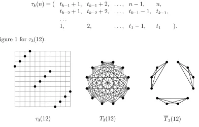
Myers [22] described a permutation τk(n) which gives an upper bound on mk(n). It
consists of k increasing sequences K whose sizes differ by at most one and every monotone sequence of length k+ 1 is entirely contained in one of the K sequences. In other words, with tj =bjn/kc, an example of such a permutation is
τk(n) = ( tk−1+ 1, tk−1+ 2, . . . , n−1, n,
tk−2+ 1, tk−2+ 2, . . . , tk−1 −1, tk−1,
. . .
1, 2, . . . , t1−1, t1 ).
See Figure 1 for τ3(12).
T3(12) T3(12)
[image:3.612.101.493.284.534.2]τ3(12)
Figure 1: Permutation τ3(12) and its representation graph (introduced in Section 2) T3(12).
Let r≡n (mod k), where 0≤r < k. It is easy to see that
mk(τk(n)) = r d
n/ke
k+ 1
+ (k−r)
b
n/kc
k+ 1
≈ 1
kk
n
k+ 1
.
Myers [22] proved that m2(n) = m2(τ2(n)) holds and he described all permutations
Conjecture 1 (Myers [22]). Let n and k be positive integers. In any permutation of [n]
there are at least mk(τk(n)) monotone subsequences of length k+ 1.
Notice that any permutation (a1, . . . , an) and its reverse (an, . . . , a1) contain the same number of monotone subsequences, only the increasing subsequences change to decreasing subsequences and vice versa. In particular, mk(τk(n)) = mk(τkR(n)), where τkR(n) denotes
the reverse of τk(n). Moreover, there might be other permutations τ such that mk(τ) =
mk(τk(n)).
As we already mentioned, Myers showed the conjecture is true fork = 2, which is actually a consequence of Goodman’s formula [15]. Very recently, Samotij and Sudakov [32] confirmed the conjecture if n ≤ k2 +ck3/2/logk for some absolute positive constant c, provided k is sufficiently large.
Subject to the additional constraint that all the monotone subsequences of length k+ 1 are either all increasing or all decreasing and n≥k(2k−1), Myers proved that every such a permutation contains at least the conjectured number of monotone subsequences of lengthk+ 1. He also gave the listWk
n of all such permutationsτ of [n] that satisfy mk(τ) =mk(τk(n)).
Every permutation from Wk
n can be decomposed into k disjoint monotone subsequences
s1, . . . , sk that are either all increasing or all decreasing and their sizes differ by at most one.
Moreover, every monotone subsequence of length k + 1 is a subsequence of sj for some j.
These permutations look similar toτk(n) orτkR(n). It turns out that there are 2 k nmodk
Ck2k−2
of them, whereCk is thekth Catalan number.
The interested reader can find the precise definition of Wk
n for generalk in [22]. Here, we
study the number of monotone subsequences withk = 3. Hence we give a simpler alternative definition for W3
n, where n≥15.
First we describe a method to get any permutation from W3
n with no increasing
subse-quence of length 4.
1. Start with the identity permutation.
2. Divide it into 3 blocks such that the size of each block is bn/3c or bn/3c+ 1. More formally, choose elements b1 and b2 such that b1, b2 −b1 and n−b2 are all from the set{bn/3c,bn/3c+ 1}. Then the three blocks are (1,2, . . . , b1), (b1+ 1, b1+ 2, . . . , b2),
(b2+ 1, b2+ 2, . . . , n). (There are 1 or 3 choices for the pair (b1, b2), depending on the
remainder of dividing n by 3.)
3. Reverse the blocks. At this point we have the permutation (b1, b1−1, . . . ,2,1, b2, b2− 1, . . . , b1 + 2, b1+ 1, n, n−1, . . . , b2+ 2, b2+ 1).
4. Change the subsequence (2,1, b2, b2 − 1) to one of the following: (2,1, b2, b2 − 1), (2, b2,1, b2−1), (2, b2, b2−1,1), (b2,2,1, b2−1), (b2,2, b2−1,1).
5. Make a similar replacement for the subsequence (b1+ 2, b1+ 1, n, n−1).
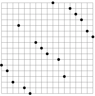
Figure 2: Permutation (6,5,3,13,2,1,10,9,8,17,7,4,16,15,14,12,11).
7. Make a similar replacement for the subsequence (b2, b2−1, b2+ 2, b2 + 1).
Each above permutation (as well as its reverse) belongs to W3
n since it has m3(τ3(n))
monotone subsequences of length 4, all of which are decreasing. For n ≥15, we exhaust all ofW3
n, as the number of obtained permutations, 2·54 3r
whereris the remainder of dividing
n by 3, coincides with the value of |W3
n| obtained by Myers.
To illustrate the above process, let n = 17. We start with (1,2, . . . ,17). Letb1 = 5, b2 = 11. After the reversal of the blocks, we have (5,4,3,2,1,11,10,9,8,7,6,17,16,15,14,13,12). Now we can change, one by one in the given order, the subsequences (2,1,11,10), (7,6,17,16), (5,4,7,6), (11,10,13,12) to (11,2,1,10), (17,7,6,16), (6,5,7,4), (13,10,12,11) respectively, to get
(6,5,3,13,2,1,10,9,8,17,7,4,16,15,14,12,11).
This permutation is depicted in Figure 2.
In his paper, Myers [22] also conjectured a weaker asymptotic version.
Conjecture 2 (Myers [22]). Let k be positive integer and let n → ∞. In any permutation of [n] there are at least (1 +o(1)) k+1n
/kk monotone subsequences of length k+ 1.
First, we prove Conjecture 2 for k = 3.
Theorem 3. Any permutation of [n] contains at least (1/27 + o(1)) n4
monotone subse-quences of length 4.
Our main result is proving Conjecture 1 for k = 3 andn sufficiently large.
Theorem 4. There exists n0 such that if n≥n0, then every permutation τ on [n] contains
at least
b
n/3c
4
+
b
(n+ 1)/3c
4
+
b
(n+ 2)/3c
4
monotone subsequences of length 4, with equality if and only if τ ∈ W3
Our results are proved using the flag algebra framework and the stability method. Al-though Theorems 3 and 4 are stated in terms of permutations, we translate them to the language of graph theory since the resulting computations and arguments are simpler. In graph theory language, we minimize the number of copies of K4 and K4 over graphs from permutations on [n]. Let us note that the question of minimizing the number of copies of
K4 and K4 over all graphs on n vertices is open. The best upper bound ≈ 1/33 is due to Thomason [36]. The first known lower bound ≈1/46 is due to Giraud [13]. It was improved using flag algebras to 0.0287... by Sperfeld [34] and independently by Nieß [23], and then further improved by Flagmatic [37] to 0.0294...≈1/34.
We also had a computer program, developed originally by Dan Kr´al, doing flag algebra, computations for permutations directly. It was easy to modify this program to compute upper bounds on densities of other subsequences instead of lower bounds for monotone subsequences. The results that we obtained will be explained in the next paragraph.
The packing density of a permutation τ ∈ Sk is the limit for n → ∞ of the maximum
density of τ in σ over all σ ∈ Sn. We denote the limit by δ(τ). The packing density is
well understood [1] for the so-calledlayered permutations1. Up to a symmetry, this includes all permutations in S3 and all but two permutations, 1342 and 2413, from S4. Albert, Atkinson, Handley, Holton, and Stromquist [1] proved that 0.19657 ≤ δ(1342) ≤ 2/9 and 51/511 ≤ δ(2413)≤ 2/9. Presutti [27] improved the lower bound for δ(2413) to 0.1024732. Further improvement on the lower bound was obtained by Presutti and Stromquist [28] who showed that 0.1047242275767320904. . . ≤ δ(2413) and conjectured that it is the correct value. A direct application of the semidefinite method from the flag algebra framework for permutations on S7 gave upper bounds δ(1342) ≤ 0.1988373 and δ(2413) ≤ 0.1047805. Since our upper bounds do not match the lower bounds, we will not discuss these bounds any further in this paper.
This paper is organized as follows. In the following section, we translate the problem of determining the density of monotone subsequences in permutations to determining densities of particular induced subgraphs in permutation graphs. In Section 3, we describe how we use the framework of flag algebras and we will prove Theorem 3. Our proof of the density result actually provides some additional information about the extremal structures, which leads to a proof of a stability property for this problem. This is discussed in Section 4. Finally, in Section 5, we use the stability property to prove Theorem 4.
We utilize the semidefinite method from flag algebras to formulate our question about subgraph densities as an optimization problem, more precisely, as a semidefinite program-ming problem. With a computer assistance, we generate this semidefinite programprogram-ming problem and then we use CSDP [8], an open-source semidefinite programming library, to find a numerical (approximate) solution to the problem. In order to obtain an exact result, the numerical solution needs to be rounded. This was done again with a computer assistance in a computer algebra software SAGE [35]. We had trouble finding a detailed description
1A permutation τ ∈[n] is layered if there exist positive numbersn
1, . . . , nr summing to n, such thatτ
starts with then1first positive integers in reverse order, followed by the nextn2 positive integers in reverse order and so on. For exampleτR
of rounding in other papers. Hence we decided to include more details about our rounding procedure in the appendix.
Our computer programs, their outputs, and their description for the flag algebra part of this paper can be downloaded athttp://www.math.uiuc.edu/~jobal/cikk/permutations/.
2
Graph Densities
Given a graphG, we use V(G) andE(G) to denote its vertex and edge sets respectively, and letv(G) =|V(G)|, e(G) = |E(G)|. For a vertexv ofG, we denote the set of its neighbors by ΓG(v). We omit a subscript, ifG is clear from the context. Given two graphs Gand G0, an isomorphism between them is a bijection f : V(G)→ V(G0) satisfying f(v
1)f(v2)∈ E(G0) if and only if v1v2 ∈ E(G). Two graphs G and G0 are isomorphic (G ∼= G0) if and only if there is an isomorphism between them. For a graph G and a vertex set U ⊆V(G), denote by G[U] the induced subgraph of G on vertex set U. Suppose H and G are graphs on l
and n vertices respectively. Let P(H, G) be the number of l-subsets U of V(G) such that
G[U]∼=H, and define the density of H in Gto be
p(H, G) = P(H, Gn )
l
.
Given a permutation τ of [n], define its representation graph to be a graph on vertex set [n] where ij with i < j is an edge if and only if τ(i) > τ(j). Call an n-vertex graph G
admissible if there is a permutation of [n] whose representation graph is isomorphic toG, so the vertex set of Gmay not be [n]. Denote byMl the set of admissible graphs onl vertices,
up to isomorphism. It is easy to see that if G is admissible, then so are G and all induced subgraphs of G.
Given a permutation τ of [n], let G be its representation graph. Then the number of monotone subsequences of length 4 in τ is equal to the number of K4’s and K4’s in G, i.e.,
m3(τ) =P(K4, G) +P(K4, G). Let
F(G) = P(K4, G) +P(K4, G) and f(G) =p(K4, G) +p(K4, G).
Instead of proving Theorem 3 directly, we prove its reformulation to the language of graphs and densities.
Theorem 5. If G is an admissible graph on n vertices, then f(G) ≥ 1/27 + o(1), where
o(1) →0 as n → ∞.
It is easy to see that
f(G) = X
H∈Ml
f(H)p(H, G) for 4≤l≤n. (1)
Therefore minH∈Mlf(H) provides a lower bound on f(G) (since 0 ≤ p(H, G) ≤ 1 and
P
Denote by T3(n) the 3-partite Tur´an graph on n vertices (i.e. complete 3-partite graph on n vertices with sizes of parts differing by at most one). We can see that T3(n) is the representation graph ofτ3(n). See Figure 1 for an example, where n= 12.
Theorem 6. There exists an n0 such that if G is an admissible graph on n ≥ n0 vertices
minimizing F over all admissible graphs on n vertices, then G is obtained from T3(n) by
removing edges or G is obtained from T3(n) by adding edges.
Remark: LetG be an extremal graph. By Theorem 6,Gcan be transformed into T3(n) or
T3(n). We may assume without loss of generality (w.l.o.g.) that G is obtained from T3(n) by removing edges. Since T3(n) does not contain any copy of K4 and removing edges does not introduce new copies of K4, there are no K4’s in G. Moreover, sinceG is extremal and removing edges does not destroy any copy of K4, the numbers of copies of K4 in G and
T3(n) are equal. Hence we know that in an extremal permutationτ, monotone subsequences of length 4 are either all increasing or all decreasing. Thus τ belongs to the family W3
n
constructed by Myers (and Theorem 4 follows from Theorem 6). In fact, it is not hard to see that τ ∈ W3
n directly. Indeed, τ can be decomposed into three monotone subsequences
s1, s2, s3, that correspond to the parts of Tur´an graph, and all monotone 4-subsequences are entirely contained in them. Then it follows that the domains of s1, s2, s3 form three consecutive intervals of [n], except some possible intertwining at their ends that involves at most two elements from each interval, which leads to the desired structure of τ.
3
Flag Algebra Settings
The flag algebra method, invented by Razborov [29], is a very general machinery and has been widely used in extremal graph theory. See [30] for a recent survey of flag algebra applications. To name just some of them: flag algebra was used for attacking the Caccetta-H¨aggkvist conjecture [19, 31], determining induced densities of graphs [10, 16, 17, 25, 26], of hypergraphs [5, 12, 14, 24], of oriented graphs [33], of subhypercubes in hypercubes [3, 7], of colored graphs in a colored environment [6, 9, 18, 20], and for attacking some problems in geometry [21].
We apply this method to the family of admissible graphs. Atype σ is an admissible graph on vertex set [k] for some non-negative integerk, where k is called thesize ofσ, denoted by
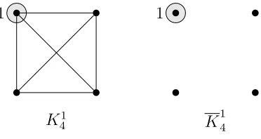
|σ|. We use 0 and 1 to denote (the unique) types of size 0 and 1 respectively. Aσ-flag F is a pair (M, θ) where M is an admissible graph and θ : [k] → V(M) induces a labeled copy of σ in M. In other words, we use [k] to label k vertices of an unlabeled graph M, and the labeled vertices induce a labeled copy of σ. Two σ-flags F1 = (M1, θ1) andF2 = (M2, θ2) are
isomorphic (denoted as F1 ∼= F2) if there exists a graph isomorphism f : V(M1)→ V(M2) such thatf θ1 =θ2. Such a function f is called a flag isomorphism fromF1 to F2. Given an admissible graphM, if allσ-flags with the underlying graph M are isomorphic, then we use
Mσ to denote this uniqueσ-flag, see Figure 3 for an example whereM ∈ {K
4, K4}. Denote by Fσ
l the set of σ-flags on l vertices, up to isomorphism. Note that Fl0 is just Ml and Fσ
1
K1
4
1
[image:9.612.217.403.71.170.2]K14
Figure 3: 1-flags K1
4 and K 1 4.
In Section 2, we defined graph densityp(H, G), which extends to flag density in a straight-forward way. Given σ-flags F ∈ Fσ
l and K = (G, θ)∈ Fnσ for l ≤ n, define P(F, K) to be
the number of l-subsets U of V(G) such that Im(θ) ⊆ U and (G[U], θ) ∼= F. Additionally, define p(F, K), the density of F inK as
p(F, K) = P(n−|σ|F, K)
l−|σ| .
By convention, we set P(F, K) = 0 if n < l. More generally, given flags F ∈ Fσ l , F
0 ∈ Fσ l0
and K = (G, θ) ∈ Fσ
n, where n ≥ l +l
0− |σ|, we define a joint density p(F, F0;K) as the
probability that if we choose two subsets U, U0 ofV(G) uniformly at random, subject to the
conditions |U|=l,|U0|=l0 and U∩U0 = Im(θ), then (G[U], θ)∼
=F and (G[U0], θ)∼
=F0. In
this paper, whenever we use p(F, K) or p(F, F0;K), we assume that the size of K is large
enough.
It is not very hard to show that (see Lemma 2.3 in [29])
p(F, K)p(F0, K) =p(F, F0;K) +o(1), (2)
where o(1) tends to 0 as n tends to infinity. Let X = [F1, . . . , Ft] be a vector of σ-flags with
Fi ∈ Flσi. For any such X and a σ-flag K define XK = [p(F1;K), . . . , p(Ft;K)]. It follows
that for any t-by-t positive semidefinite matrix Q={Qij}, we have
0≤XT
KQXK = X
ij
Qijp(Fi;K)p(Fj;K) = X
i,j
Qijp(Fi, Fj;K) +o(1). (3)
In the definition of p(F, K) and p(F, F0;K), we require F, F0 and K to be σ-flags, but the
definition itself extends to the case where F, F0 are σ-flags but K is not. In this case, by
the definition, we have p(F, K) = p(F, F0;K) = 0. Let Θ(k, G) be the set of all injective
mappings from [k] to V(G) where Gis an admissible graph. We can extend (3) to any θ∈Θ(|σ|, G):
0≤X i,j
Therefore, if we choose θ from Θ(|σ|, G) uniformly at random, then its expectation is non-negative:
0≤X i,j
Eθ∈Θ(|σ|,G)[Qijp(Fi, Fj; (G, θ))] +o(1)
= X
H∈Ml
X
i,j
Eθ∈Θ(|σ|,H)[Qijp(Fi, Fj; (H, θ))] !
p(H, G) +o(1).
(Recall that we assumed that l≥2li− |σ| for eachi.) Note that the coefficient of p(H, G) is
determined byσ, X, Q andH. In particular, it is independent ofG, so denote this coefficient
bycH(σ, X, Q). Then we have
X
H∈Ml
cH(σ, X, Q)p(H, G) +o(1)≥0.
Every choice of σ, X, Q gives one such inequality. We can add the inequalities obtained for several different typesσi, using appropriateXi andQi. DenotingcH =
P
icH(σi, Xi, Qi),
we obtain
X
H∈Ml
cH ·p(H, G) +o(1)≥0.
Then together with (1) we have
f(G) +o(1)≥ X
H∈Ml
(f(H)−cH)·p(H, G)≥ min H∈Ml
(f(H)−cH). (4)
By (4), if for some choice of (large enough) l and cH we have
min
H∈Ml
(f(H)−cH) = 1/27, (5)
then we would prove Theorem 5.
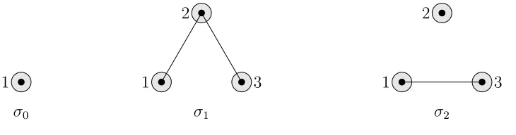
Proof of Theorem 5. We show (5) with l = 7, where |M7| = 776. We use three choices of
(σ, X, Q). We use types σ0 : P1, σ1 : P3, and σ2 : P3, where Pi is a path on i vertices, see
Figure 4.
For σ0, X0 consists of flags in F4σ0, for σi with i= 1,2, Xi consists of flags in F5σi. Here we have |Fσ0
4 | = 20 and |F5σ1| = |F5σ2| = 71. As we already mentioned, the flag algebra method is computer assisted. We use a computer program to findM7,F4σ0,F
σ1
5 ,F
σ2
5 , and to compute Eθ p(F, F0; (H, θ)) for each H ∈ My. Then finding positive semidefinite matrices
Q0, Q1, Q2 to maximize minH∈M7(f(H)− cH) can be done by computer solvers such as
CSDP [8] and SDPA [38]. Unfortunately, solvers can only give an approximate solution. For this problem, we get 0.0370370369999. In order to get exactly 1/27, we need to round the matrices Q0, Q1, Q2 found by a computer solver. By rounding we mean finding rational matrices Q0
1
σ0
1 3
2
σ1
1 3
2
[image:11.612.128.493.71.167.2]σ2
Figure 4: Types used in flag computation.
To simplify the process of rounding, we reduce the number of variables and constraints by restricting the set of feasible solutions. Fori∈ {1,2,3}and flagsF1, F2 denote by Qi(F1, F2) the entry in Qi corresponding to indices of F1 and F2 in Xi. Since f(H) = f(H) for every
graph H, a natural restriction is that
f(H)−cH =f(H)−cH (6)
for every graph H. This will allow us to consider only one of H, H and thus decrease the number of constraints from 776 to 388 since there is no self-complementary graph on 7 vertices as the number of possible edges and non-edges is 72
= 21 which is an odd number. Since σ1 = σ2, we add the constraints Q1(F1, F2) = Q2(F1, F2) for every F1, F2 ∈ F5σ1. This makes Q2 completely defined by Q1. Moreover, we add the constraints Q0(F1, F2) =
Q0(F1, F2) = Q0(F1, F2) = Q0(F1, F2) for every F1, F2 ∈ F4σ0. This reduces the number of entries to round in the symmetric matrix Q0 from 212
to 112
.
We reduced the number of constraints from 776 to 388, and we reduced the number of variables from 212
+ 2 722
to 112
+ 722
. With these reductions, we managed to round the entries in Q1, Q2 and Q3 and thus we obtained a solution for (5).
The rounded matrices as well as programs computing all possible X and performing the rounding process can be obtained athttp://www.math.uiuc.edu/~jobal/cikk/permutations/.
We give more details about the rounding step in the appendix.
In (5), we not only have that the minimum off(H)−cH is 1/27, which proves Theorem 5,
but we also have the values of f(H)−cH for each H inM7.
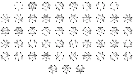
LetL ={H ∈ M7 :f(H)−cH = 1/27}. We listed L in Figure 5. We have the following
proposition for graphs not inL.
Proposition 7. Let G be an admissible graph of order n→ ∞ such that f(G) = 271 +o(1). If H ∈ M7\ L, then p(H, G) = o(1).
Proof. Using (4), we have that
1
27+o(1) =f(G) +o(1)≥
X
H∈Ml
In this section, we showed that by choosingl= 7 and typesσ0, σ1, σ2we have minH∈M7(f(H)−
cH) = 1/27. Then since P
H∈Mlp(H, G) = 1, we know that if f(H)−cH > 1/27, then p(H, G) = o(1).
Notice that the Proposition 7 can be stated equivalently as follows.
Proposition 8. For every δ > 0 there exists n0 = n0(δ) and ε0 > 0 such that for every
admissible graphG of ordern > n0 withf(G)<1/27 +ε0, ifH ∈ M7\ L, thenp(H, G)< δ.
Note that it is sufficent to pick
ε0 < δ· min
H∈M7\L{f(H)−cH −1/27}.
Proposition 8 will help us to get the stability property of admissible graphs G with
[image:12.612.78.534.260.521.2]f(G) = 271 +o(1), which is discussed in the next section.
Figure 5: Graphs in L. The first eight graphs are induced subgraphs of T3(n) orT3(n). In order to save space, a depicted graphH represents both H and H.
4
Stability Property
In this section we will prove the following stability type statement.
Theorem 9. For every ε > 0 there exist n0 and ε0 >0 such that every admissible graph G
of order n > n0 with f(G) ≤ 271 +ε0, is isomorphic to either T3(n) or T3(n) after adding
We will use our flag algebra results from Section 3 and the infinite removal lemma to prove Theorem 9. The infinite removal lemma, proved by Alon and Shapira [2], is a substantial generalization of the induced removal lemma.
Lemma 10 (Infinite Removal Lemma [2]). For any (possibly infinite) family H of graphs
and ε > 0, there exists δ > 0 such that if a graph G on n vertices contains at most δnv(H)
induced copies of H for every graph H in H, then it is possible to make G induced H-free, for every H ∈ H, by adding and/or deleting at most εn2 edges.
Proof of Theorem 9. Fix an ε > 0. Let δ be from Lemma 10, when applied with ε and
H= (M7\ L)∪ {not admissible graphs}. Let ε0 < ε4 and n1 be given by Proposition 8 such
thatp(H, G)< δ for everyH ∈ M7\ L andG on at leastn1 vertices. Letn0 > n1 such that
f(G)>1/27−ε0 for all Gof order at least n
0/2. Notice that every non-admissible graph H satisfies p(H, G) = 0 for every admissible G.
Let G be an admissible graph of order n > n0 with f(G) ≤ 271 +ε0. Now we apply Lemma 10 and conclude that by adding and/or deleting at most εn2 edges, every induced subgraph of G on 7 vertices belongs to L and G is still admissible.
By direct inspection of graphs in L, we have the following two properties of G. Notice that if all 7-vertex induced subgraphs ofGsatisfy these two properties, then so doesG. Also notice that a graph H satisfies these two properties if and only if H satisfies them.
Property A: There are noK4 and K4 that share a vertex.
Property B: For every pair ofK4’s that share at least one vertex, the union of their vertex sets spans a clique. For every pair ofK4’s that share at least one vertex, the union of their vertex sets spans an independent set.
Let (G, x) be the 1-flag where vertex x is the labeled vertex, then P(K1
4,(G, x)) is the number of K4’s in G that contain x. Define
F(x, G) = P(K41,(G, x)) +P(K14,(G, x)) and f(x, G) = F(x, G)
v(G)−1
3
.
Then we havef(G) = (P
xf(x, G))/v(G). LetG0 =G. For i≥0, letxi be the vertex with
largest f(xi, Gi). If f(xi, Gi) > 1/27 + 2ε0/ε, we create Gi+1 from Gi by removing vertex
xi. If f(xi, Gi) ≤ 1/27 + 2ε0/ε, we define G0 = Gi and d = i. Note that f(Gi) ≤ f(Gi−1), so f(Gi)≤ f(G)≤1/27 +ε0. Also notice, that the process is not deterministic if there are
more candidates for xi for somei (any choice of xi will work).
Claim 11. d < εn.
Proof. Denote v =v(Gi−1) and y the vertex deleted fromGi−1. Then
f(Gi−1)−f(Gi)≥
4ε0
which follows from the following computation
f(Gi−1)−f(Gi) = P
xf(x, Gi−1)
v −
P
xf(x, Gi)
v −1
= f(y, Gi−1) +
P
x6=yf(x, Gi−1)
v −
P
xf(x, Gi)
v−1
= f(y, Gi−1) + (
P
x6=yF(x, Gi−1))/ v−1
3
v −
P
xf(x, Gi)
v−1
= 4f(y, Gi−1) +
v−2 3
(P
xF(x, Gi))/( v−2 3 v−1 3 ) v − P
xf(x, Gi)
v−1
= 4f(y, Gi−1) +
v−4
v−1
P
xf(x, Gi)
v −
P
xf(x, Gi)
v−1
= 4(v−1)f(y, Gi−1) + (v−4)
P
xf(x, Gi)−v P
xf(x, Gi)
v(v−1)
= 4f(y, Gi−1)−4f(Gi)
v
≥ 4 (2ε
0/ε−ε0)
n ≥
4ε0
εn.
If follows from n ≥ n0 that f(H) > 1/27−ε0 for every admissible graph H on at least
n/2 vertices. However, if d > εn, then for i =εn, f(Gi)<1/27 +ε0−4iε0/εn <1/27−ε0,
which is a contradiction sinceGi has at least n−εn= (1−ε)n ≥n/2 vertices.
Claim 12. The number of verticesxwith f(x, G0)< 1
27−εis at mostεv
0, wherev0 =v(G0).
Proof. Let the number of vertices with f(x, G0)< 1
27−ε be z.
v0f(G0) =X
x
f(x, G0)< z
1 27−ε
+ (v0−z)
1 27+
2ε0
ε
=−zε+v0 1
27+v
02ε0
ε −z
2ε0
ε < v0
27 + 2v0ε0
ε −εz.
If z > εv0, then we get
f(G0)< 1
27 + 2ε0
ε −ε
2 < 1 27−ε
0
,
which is a contradiction (recall that ε0 < ε4).
Let G00 be the graph obtained from G0 by removing all such vertices. We removed at
most εv0 vertices, so
F(x, G0)−F(x, G00)< εv0
v0−2
2
for each vertexx∈V(G00). Denote v(G00) by v00. We havev00 ≥(1−ε)v0 and
F(x, G00)> F(x, G0)−εv0
v0−2
2
≥
1 27 −ε
v0 −1
3
−εv0
v0−2
2
≥
1 27 −ε
(v0−1)(v0 −2)(v0−3)
6 −ε
(v0−1)(v0−2)(v0−3)
1.5
≥
1 27 −5ε
v00−1
3
.
We know that f(x, G0)≤1/27 + 2ε0/ε. Then since ε0 < ε4 and v00 ≥(1−ε)v0, we have
F(x, G00)≤F(x, G0)≤
1 27 +
2ε0
ε
v0−1
3
≤
1 27+ 5ε
v00−1
3
.
This means that for every vertex x∈V(G00), we have
1 27−5ε
v00−1
3
< F(x, G00)<
1 27 + 5ε
v00−1
3
. (8)
For x, y ∈ V(G00), write x ∼ y if x = y or there is a chain of vertex-intersecting K
4’s or K4’s connecting x to y. Clearly, ∼ is an equivalence relation, and by Property A, each chain consists of cliques only or independent sets only. By Property B, each ∼-equivalence class is a clique or an independent set. Let s be the size of the class of x. This means that
F(x, G00) = s−1 3
. It follows from (8) that
1 3 −16ε
v00< s <
1 3 + 16ε
v00, (9)
which means each∼-equivalence class has size at least (1/3−16ε)v00and at most (1/3+16ε)v00.
Next, we claim that equivalence classes are all cliques or all independent sets. Suppose on the contrary that G00[A] is a clique and G00[B] is an independent set. W.l.o.g., assume
that the edge density between A and B is at least 1/2. Then there exists a vertex x in B
such that |Γ(x)∩A| ≥ |A|/2. Taking a 4-setX ⊂B containingx and a 3-setY ⊂Γ(x)∩A, then G00[X] = K
4 and G00[Y ∪ {x}] = K4. We find a K4 and a K4 that share a vertex x, contradicting Property A.
W.l.o.g., assume that each equivalence class is an independent set. It follows from (9) that there are exactly three equivalence classes. Denote them by A1, A2 and A3. If there exist an x ∈ Ai and y1, y2, y3 ∈ Aj (i 6= j) such that none of xyk is an edge, then x ∼ yk,
which would contradict Property B. This means that all but at most 4v00 of edges between
equivalence classes are in G00. To get T
3(v00), we need to add these edges and balance the three sets. In this step we change at most 4n+ 16εn2 edges.
We first change at most εn2 edges of G such that G does not contain anyH ∈ M 7 \ L, then we remove at most 2εn vertices to form G00. Then we change at most 4n + 16εn2 edges to get T3(v00). Therefore, to get T3(n) from G, we only need to change at most
5
Exact Result
We call u∈V(G) aclone ofv ∈V(G) if Γ(u) = Γ(v). In particular, uv is not an edge ofG.
Proposition 13. Let G be an admissible graph of order n. If we add a clone x0 of some
x ∈ V(G) to form a new graph G0 of order n+ 1, i.e., Γ
G0(x0) = ΓG(x), then G0 is still
admissible.
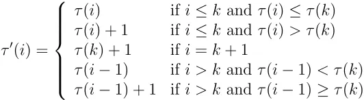
Proof. The graphGcomes from some permutationτ on [n]. Letk be the number in [n] that corresponds to x, then we can construct a new permutation τ0 on [n+ 1] as follows:
τ0(i) =
τ(i) if i≤k and τ(i)≤τ(k)
τ(i) + 1 if i≤k and τ(i)> τ(k)
τ(k) + 1 if i=k+ 1
τ(i−1) if i > k and τ(i−1)< τ(k)
τ(i−1) + 1 if i > k and τ(i−1)≥τ(k).
The representation graph of τ0 is G0 with k+ 1 corresponding to the new vertex x0.
Let S be the 7-vertex graph obtained by gluing three paths xyizi, i = 1,2,3, at the
common vertexx, see Figure 6.
x
y1 z1
y2
z2
y3
z3
[image:16.612.168.434.213.286.2]S
Figure 6: The graph S.
Proposition 14. The graph S is not admissible.
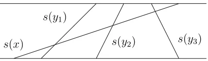
Proof. Admissible graphs can be alternatively defined as intersection graphs of segments whose endpoints lie on two parallel lines. For a vertex v in S denote by s(v) the segment representing v. Since y1, y2 and y3 form an independent set, segments representing them do not intersect. On the other hand s(x) intersects all of them. W.l.o.g., assume that s(y2) is middle of the three segments in the order they intersect s(x), see Figure 7. Since z2 is adjacent only to y2, the segment representing z2 intersects only s(y2), which is clearly impossible.
s(y1)
s(y2) s(y3)
[image:17.612.200.414.69.132.2]s(x)
Figure 7: Representation of part of S as intersecting segments.
Proof of Theorem 6. Let G be an admissible graph of order n with minimum F among all admissible graphs on n vertices, wheren is sufficiently large. Fixε >0 sufficiently small. In particular, by Theorem 5, we assumenlarge enough such thatf(G)≤ 271 +ε. LetV =V(G). By Theorem 9, we also assume that we can makeGequal to T3(n) by adding/or deleting at most εn2 edges (also largen needed). Take a complete 3-partite graph T on V such that
|W| is minimized, where W = E(T)4E(G). From Theorem 9 we know that |W| < εn2 and V can be partitioned into V1, V2, V3 of sizes (1/3−ε)n < |Vi| < (1/3 +ε)n, which are
the parts ofT. Let B =E(G)\E(T) andM =E(T)\E(G). We call edges in B bad, in M
missing, and in W wrong.
Proposition 15. For any x∈V we have f(x, G)≤1/27 + 3 2ε.
Proof. First we prove that for any x, y ∈V we have
|F(x, G)−F(y, G)| ≤
n−2
2
. (10)
W.l.o.g., assume F(x, G)≥F(y, G). Let G0 be obtained fromG by adding a clone of y and
removing x. By Proposition 13,G0 is an admissible graph. By the extremality of Gwe have
0≤F(G0)−F(G)≤F(y, G)−F(x, G) +
n−2
2
,
which gives (10).
Recall, that F(G) = 1 4
P
x∈V F(x, G) ≤ F(T3(n)). Suppose that there exists an x such
that f(x, G)>1/27 + 32ε, i.e.
F(x, G)>
1 27+
3 2ε
n−1
3
.
By using (10) we have that for everyy ∈V
F(y, G)>
1 27+
3 2ε
n−1
3
−
n−2
2
>
1 27 +ε
n−1
3
.
Hence f(G)> 1
27+ε which contradicts our assumption that f(G)≤ 1 27 +ε.
Proof. Let x be a vertex in V. Let αi = |Γ(x)∩Vi|/|Vi| where V1, V2, V3 are the parts of
T. Let δ = 2ε1/6. If every α
i ∈ (δ,1− δ) then there are at least δ6(13 −ε)6n6 ways to
choose a set U ={y1, y2, y3, z1, z2, z3} with yi ∈ Vi\Γ(x)−x and zi ∈ Vi∩Γ(x)−x. The
number of such sets U which contain a wrong edge is at most n
4
|W| < εn6/24. Since
δ6(1 3 −ε)
6n6 > εn6/24, there exists U that does not contain any edge of W, which means
U ∪ {x} induces the complement of the non-admissible graph S in G, a contradiction to Proposition 14.
W.l.o.g., we may assume that α1 < δ orα1 >1−δ.
If α1 < δ, then the number of copies of K4 via x whose other three vertices are in A1 is
at least
(1−δ)(1/3−ε)n
3
≥(1−δ)3
1 3 −ε
3 n 3 ≥ 1
27−ε−δ
n
3
.
Thus x has to be connected to almost every vertex in A2 ∪A3. To be more precise, assume αi ≤1−η for fori= 1 or i= 2. Then we should have
η(1/3−ε)n
3
≤
(1−αi)|Vi|
3
<
1 27+ε
n 3 − 1
27 −ε−δ
n
3
. (11)
However, (11) does not hold since η= 2ε1/18, so we know that α
2 >1−η and α3 >1−η. If α1 >1−δ, then
f(x, G)≥
3
X
i=1
(1−αi)|Vi|
3
+α1α2α3|V1||V2||V3| −εn3
!, n 3 ≥
(1−α2)|V2| 3
+
(1−α3)|V3| 3
+ (1−δ)α2α3|V1||V2||V3| −εn3
n
3
= (1/3−ε)3 (1−α2)3 + (1−α3)3+ 6(1−δ)α2α3
−6ε
≥(1/3−ε)3 (1−α2)3+ (1−α3)3+ 5α2α3
−6ε.
Leth(x, y) = (1−x)3+ (1−y)3+ 5xy. The minimum value of the polynomialh(x, y) on [0,1]2 is 1 with equality if and only if {x, y}= {0,1}. We know that f(x, G) ≤ 1/27 + 3
2ε. Then by the continuity ofhand the compactness of [0,1]2,{α
2, α3}is close to{0,1}. W.l.o.g., assume α2 is close to 1 and α3 is close to 0. Let γ = 6ε1/3. If α2 ≤1−γ or α3 ≥γ, then
f(x, G)≥(1/3−ε)3 (1−α2)3+ (1−α3)3+ 5α2α3
−6ε.
= (1/3−ε)3(1 + (2−5(1−α2))α3+ 3α23−α33+ (1−α2)3)−6ε
≥(1/3−ε)3(1 +α3+ (1−α2)3)−6ε
> 1
27 + 3 2ε,
which is a contradiction with Proposition 15. Soα2 >1−γ and α3 < γ.
It follows from Lemma 16 that every bad edge xy ∈ B belongs to at least (1/9−η)n2 copies of K4, because
1 3 −ε
2
n2−2ηn
1 3 +ε
n= 1 9− 2 3ε+ε
2− 2η
3 −2ηε
n2 ≥
1 9 −η
n2.
On the other hand, if we remove xyfromE(G), this would create at most (1/18 +η2)n2 copies of K4, because
(1/3 +ε)n
2 + ηn 2 ≤ 1 18+ ε 3+ ε2 2 + η2 2
n2 ≤
1 18 +η
2
n2.
Also, by ∆(B)< ηn and b =|B|< ηn2, the number of 4-sets that contain at least two bad edges is at most
b
2
+ 2b(ηn)n≤ b
2
2 + 2ηbn
2 < ηbn2
2 + 2ηbn
2 <3ηbn2.
Thus if G0 is obtained from G by removing all bad edges of G, it satisfies F(G0)−F(G)≤ −bn2/18 +εbn2 <0 unlessb = 0, because
F(G0)−F(G)≤
1 18+η
2
bn2 −
1 9−η
bn2−6·3ηbn2
≤
− 1
18+η
2+ 19η
bn2 ≤ −bn
2
100.
Clearly, the complete 3-partite graph T can be obtained from G0 by adding all missing
edges between parts. Thus we have P(K4, T) ≤ P(K4, G0). Then since P(K4, T) = 0 ≤
P(K4, G0), the admissible graph T satisfies F(T) ≤ F(G0) < F(G) unless b = 0. By the choice of G, we have F(G) ≤ F(T), so b = 0, which means G is a subgraph of T and G
is a 3-partite graph. Then since F(G) ≤ F(H) for every H ∈ Mn, we know that G is a subgraph of T3(n) and F(G) = F(T3(n)).
6
Conclusion
In Theorem 4, we verified Conjecture 1 for k = 3 and n sufficiently large, and we fully characterized the set of the extremal configurations. While revising our paper, we discovered that using a slightly refined set-up of the flag algebra framework, we can also prove an analogue of Theorem 3 for k = 4 and k = 5. We address these two cases in a forthcoming note.
Acknowledgement
Treglown for fruitful discussions. We also thank the anonymous referees for carefully reading the manuscript and for their valuable comments, which greatly improved the presentation of the results.
References
[1] M. H. Albert, M. D. Atkinson, C. C. Handley, D. A. Holton, and W. Stromquist. On packing densities of permutations. Electron. J. Combin., 9(1):Research Paper 5, 20, 2002.
[2] N. Alon and A. Shapira. A characterization of the (natural) graph properties testable with one-sided error. SIAM J. Comput., 37(6):1703–1727, 2008.
[3] R. Baber. Tur´an densities of hypercubes. Submitted.
[4] R. Baber. Some results in extremal combinatorics. Dissertation, 2011.
[5] R. Baber and J. Talbot. Hypergraphs do jump. Combin. Probab. Comput., 20(2):161– 171, 2011.
[6] R. Baber and J. Talbot. A solution to the 2/3 conjecture. SIAM J. Discrete Math., 28(2):756–766, 2014.
[7] J. Balogh, P. Hu, B. Lidick´y, and H. Liu. Upper bounds on the size of 4- and 6-cycle-free subgraphs of the hypercube. European Journal of Combinatorics, 35:75–85, 2014.
[8] B. Borchers. CSDP, A C library for semidefinite programming. Optimization Methods and Software, 11(1-4):613–623, 1999.
[9] J. Cummings, D. Kr´al, F. Pfender, K. Sperfeld, A. Treglown, and M. Young. Monochro-, matic triangles in three-coloured graphs. J. Combin. Theory Ser. B, 103(4):489–503, 2013.
[10] S. Das, H. Huang, J. Ma, H. Naves, and B. Sudakov. A problem of Erd˝os on the minimum number of k-cliques. J. Combin. Theory Ser. B, 103(3):344–373, 2013.
[11] P. Erd˝os and G. Szekeres. A combinatorial problem in geometry. Compositio Math., 2:463–470, 1935.
[12] V. Falgas-Ravry and E. R. Vaughan. Applications of the semi-definite method to the Tur´an density problem for 3-graphs. Combin. Probab. Comput., 22(1):21–54, 2013.
[14] R. Glebov, D. Kr´al, and J. Volec. A problem of Erd˝os and S´os on 3-graphs. In, The Seventh European Conference on Combinatorics, Graph Theory and Applications, vol-ume 16 of CRM Series, pages 3–8. Ed. Norm., Pisa, 2013.
[15] A. W. Goodman. Sur le problme de goodman pour les quadrangles et la majoration des nombres de ramsey. The American Mathematical Monthly, 66(9):778–783, 1959.
[16] A. Grzesik. On the maximum number of five-cycles in a triangle-free graph. J. Combin. Theory Ser. B, 102(5):1061–1066, 2012.
[17] H. Hatami, J. Hladk´y, D. Kr´al, S. Norine, and A. Razborov. On the number of pentagons, in triangle-free graphs. J. Combin. Theory Ser. A, 120(3):722–732, 2013.
[18] H. Hatami, J. Hladk´y, D. Kr´al, S. Norine, and A. Razborov. Non-three-colourable, common graphs exist. Combin. Probab. Comput., 21(5):734–742, 2012.
[19] J. Hladk´y, D. Kr´al, and S. Norine. Counting flags in triangle-free digraphs. In, Euro-pean Conference on Combinatorics, Graph Theory and Applications (EuroComb 2009), volume 34 of Electron. Notes Discrete Math., pages 621–625. Elsevier Sci. B. V., Ams-terdam, 2009.
[20] D. Kr´al, C.-H. Liu, J.-S. Sereni, P. Whalen, and Z. B. Yilma. A new bound for the 2, /3 conjecture. Combin. Probab. Comput., 22(3):384–393, 2013.
[21] D. Kr´al, L. Mach, and J.-S. Sereni. A new lower bound based on Gromov’s method of, selecting heavily covered points. Discrete Comput. Geom., 48(2):487–498, 2012.
[22] J. S. Myers. The minimum number of monotone subsequences. Electron. J. Combin., 9(2):RP 4, 17 pp., 2002/03. Permutation patterns (Otago, 2003).
[23] S. Nieß. Counting monochromatic copies of K4: a new lower bound for the Ramsey multiplicity problem. Submitted.
[24] O. Pikhurko. The minimum size of 3-graphs without a 4-set spanning no or exactly three edges. European J. Combin., 32(7):1142–1155, 2011.
[25] O. Pikhurko and A. Razborov. Asymptotic structure of graphs with the minimum number of triangles. E-print arXiv:1204.2846.
[26] O. Pikhurko and E. R. Vaughan. Minimum number ofk-cliques in graphs with bounded independence number. Combin. Probab. Comput., 22(6):910–934, 2013.
[27] C. B. Presutti. Determining lower bounds for packing densities of non-layered patterns using weighted templates. Electron. J. Combin., 15(1):RP 50, 10, 2008.
[29] A. A. Razborov. Flag algebras. Journal of Symbolic Logic, 72(4):1239–1282, 2007.
[30] A. A. Razborov. Flag Algebras: An Interim Report. InThe Mathematics of Paul Erd˝os II, pages 207–232. Springer, 2013.
[31] A. A. Razborov. On the Caccetta-H¨aggkvist conjecture with forbidden subgraphs. J. Graph Theory, 74(2):236–248, 2013.
[32] W. Samotij and B. Sudakov. On the number of monotone sequences. Submitted.
[33] K. Sperfeld. The inducibility of small oriented graphs. Submitted.
[34] K. Sperfeld. On the minimal monochromatic K4-density, 2011.
[35] W. Stein et al.Sage Mathematics Software (Version 5.6). The Sage Development Team, 2013. http://www.sagemath.org.
[36] A. Thomason. A disproof of a conjecture of Erd˝os in Ramsey theory. J. London Math. Soc. (2), 39(2):246–255, 1989.
[37] E. R. Vaughan. Flagmatic (version 2.0), 2013. http://www.flagmatic.org.
A
Rounding approximate solutions to exact solutions
Recall from the proof of Theorem 5 that a solution consists of several positive semidefinite matrices. For example, in our problem, our solution consists of three matrices Q0, Q1 and
Q2. For simplicity, when describing the rounding procedure, we assume that there is only one matrix. A computer solver can only solve a semidefinite program numerically and thus we get an approximate solution. Let Q be a t-by-t matrix computed by a computer solver. To make the solution exact, we need to convert entries in the matrix to rational numbers. A resulting rounded matrix Q0 must satisfy the following.
Goal 1. Q0 is positive semidefinite.
Goal 2. Q0 gives us the desired number, i.e., see (5).
The idea of the rounding is following. For most of entries in Q0 we use a rational number
close to the corresponding entry in Q. The other entries in Q0 will be computed such that
Q0 satisfies Goals 1 and 2.
We will construct a system of linear equations whose variables are entries ofQ0 (ignoring
the entries below the main diagonals) and all constants are rational numbers. There are two types of linear equations in the system, Type 1 and Type 2, which make our solution achieve Goal 1 and Goal 2 respectively. We again use computer solver to solve the linear system, but unlike a semidefinite program, a system of linear equations can be solved over rationals. When we use an entry fromQ, it is sufficient in our case if the corresponding entry in Q0
differs by at most ε= 10−5.
To achieve Goal 1, we want all eigenvalues to be non-negative. We know thatQis positive semidefinite, so all its eigenvalues are non-negative. If an eigenvalue of Q is a large positive number compared to ε, then we expect it to be still positive after rounding, since as we mentioned above, entries of Q are perturbed just a little bit. But if an eigenvalue of Q is small, for example, 10−6, then it may become −10−8 after rounding and Q0 would not be
positive semidefinite. To avoid this, we force such eigenvalues to become 0 after rounding. We do this by adding a constraint to our linear system for every such eigenvalue. Let {Xi}
be the set of eigenvectors of Q whose eigenvalues are smaller than ε1 for some ε1 >0. We assume thatXi is close to an eigenvector ofQ0 with eigenvalue 0. So we find an approximate
basis {X0
i} of the linear space generated by {Xi}, and add Q0Xi0 = 0 to our linear system.
These are Type 1 linear equations. Note that entries of Q0 are variables, so this gives us t
linear equations for eachX0
i. LetXi = [xi,1, . . . , xi,t]. The algorithm of finding Xi0 is outlined
below, which is taken from Baber’s Thesis [4]:
For each Xi:
Let` be arg maxj|xi,j|.
Set Xi =Xi/xi,`.
For all k6=i:
Set Xk =Xk−xk,`·Xi.
Guess X0
More details of the algorithm are in Section 2.4.2.2 of [4]. The last step of the algorithm means that Xi should look good and one can see instantly fromXi what the exact value is.
For example, if one sees 0.33333332, then 1/3 should be guessed.
To achieve Goal 2, we check values of f(H)−cH for all H inMl. If f(H)−cH is much
larger than 1/27, we hope that it will be still larger than 1/27 after rounding. However, if f(H)−cH is close to 1/27, a small change on entries of Q could result in f(H)−cH
being less than 1/27, which violates Goal 2. To prevent this, we add a linear equation
f(H)−cH = 1/27 for every H ∈ Ml if f(H)−cH < 1/27 +ε2 for some ε2 >0. These are Type 2 linear equations.
The system of k Type 1 and Type 2 linear equations can be written as
Ay=b,
where y = {y1, . . . , ym} corresponds to entries of Q0, A ∈ Qk×m, and b ∈ Qk. Usually, m
is larger than r = rank(A). W.l.o.g., assume that the first r columns of A are linearly independent. Then A can be written as
A0 A00
where A0 is the first r columns of A and
A00 is the rest of the columns ofA. Let y0 ={y
1, . . . , yr}and y00 ={yr+1, . . . , ym}. We assign
to yi iny00 a rational number, such that |yi −xi|< ε3, where xi ∈Q corresponds to yi and
ε3 > 0. This step can be done arbitrarily. For example, let ε3 = 10−5 and keep the first 5 digits of xi. Then we have the following matrix equation:
A0y0 =b−A00y00. (12)
Note that the number of equations in (12) may be larger than r. So this system may have no solution. But if it has a solution, then this solution is unique, which gives a matrix over rational numbers. Then we need to verify if this matrix satisfies Goals 1 and 2. If yes, we get Q0. If not, we can try to redo the computation with a smaller ε
3, or look which of the goals is violated and enlarge ε1 or ε2 to add more equations to the linear system.
If we are unlucky that the linear system (12) has no solution, then it means we added too many equations. Note that we pick eigenvalues that are smaller than ε1 and add corre-sponding Type 1 equations, and pickH with f(H)−cH <1/27 +ε2 and add corresponding Type 2 equations. In order to have fewer equations, we may re-pick Type 1 and Type 2 equations with smaller ε1 and ε2.
So far in our rounding procedure, we get Type 1 and Type 2 equations only from Q. If the attacked problem has conjectured extremal structures, we can also get Type 1 and Type 2 equations from those structures.
Take our problem for example. Let G be an extremal graph on n vertices. By Proposi-tion 7, if p(H, G) > o(1), then f(H)−cH = 1/27, which gives Type 2 equations. For our
problem, this gives the first eight graphs in Figure 5. Unsurprisingly, every H of these eight graphs satisfy f(H)−cH ≈ 1/27 in Q. So these Type 2 equations are usually generated
fromQ by the process described before. For Type 1 equations, using (4), we have
1/27 +o(1) =f(G) +o(1) ≥ X H∈M7
and
f(G)− X
H∈M7
cHp(H, G) = X
H∈M7
(f(H)−cH)·p(H, G)≥ min
H∈M7(f(H)−cH) = 1/27.
This givesP
H∈M7cHp(H, G) =o(1). Recall from Section 3 that we use (σi, Xi, Qi) to getcH.
Denote Xi ={Fji}. For θ ∈Θ(|σi|, G), let Yi,θ be the vector whose entries are p(Fji,(G, θ)).
It follows from (3) and the definition of cH that
o(1) = X
H∈M7
cHp(H, G) = X
i
Eθ∈Θ(|σi|,G)Y
T
i,θ·Qi·Yi,θ. (13)
For each θ ∈Θ(|σi|, G) we have a vector Yi,θ, but if the conjectured extremal structures
are symmetric in some sense, then there may be only C differentYi,θ’s whereC is a constant
independent of n. Choose θ from Θ(|σi|, G) uniformly at random. If P[Yi,θ = Yi,φ] > o(1)
for some φ ∈ Θ(|σi|, G), then we have Yi,φT ·Qi ·Yi,φ = 0, otherwise we do not have (13).
Since Qi 0, this means thatYi,φ is an eigenvector of Qi with eigenvalue 0, giving us Type
1 equations. In our problem, the vectors{Yi,φ}we get from conjectured extremal structures
are in the space generated by {X0
i}. So there is no need to combine equations generated