warwick.ac.uk/lib-publications
Original citation:
Das Choudhury, Sruti and Tjahjadi, Tardi. (2016) Clothing and carrying condition invariant
gait recognition based on rotation forest. Pattern Recognition Letters, 80. pp. 1-7.
Permanent WRAP URL:
http://wrap.warwick.ac.uk/79261
Copyright and reuse:
The Warwick Research Archive Portal (WRAP) makes this work by researchers of the
University of Warwick available open access under the following conditions. Copyright ©
and all moral rights to the version of the paper presented here belong to the individual
author(s) and/or other copyright owners. To the extent reasonable and practicable the
material made available in WRAP has been checked for eligibility before being made
available.
Copies of full items can be used for personal research or study, educational, or not-for-profit
purposes without prior permission or charge. Provided that the authors, title and full
bibliographic details are credited, a hyperlink and/or URL is given for the original metadata
page and the content is not changed in any way.
Publisher’s statement:
© 2016, Elsevier. Licensed under the Creative Commons
Attribution-NonCommercial-NoDerivatives 4.0 International
http://creativecommons.org/licenses/by-nc-nd/4.0/
A note on versions:
The version presented here may differ from the published version or, version of record, if
you wish to cite this item you are advised to consult the publisher’s version. Please see the
‘permanent WRAP URL’ above for details on accessing the published version and note that
access may require a subscription.
Sruti Das Choudhury, Tardi Tjahjadi
School of Engineering, University of Warwick Gibbet Hill Road, Coventry, CV4 7AL, United Kingdom.
Abstract
This paper proposes a gait recognition method which is invariant to maximum number of challenging factors of gait recognition
mainly unpredictable variation in clothing and carrying conditions. The method introduces an averaged gait key-phase image
(AGKI) which is computed by averaging each of the five key-phases of the gait periods of a gait sequence. It analyses the AGKIs
using high-pass and low-pass Gaussian filters, each at three cut-offfrequencies to achieve robustness against unpredictable variation
in clothing and carrying conditions in addition to other covariate factors, e.g., walking speed, segmentation noise, shadows under
feet and change in hair style and ground surface. The optimal cut-offfrequencies of the Gaussian filters are determined based
on an analysis of the focus values of filtered human subject’s silhouettes. The method applies rotation forest ensemble learning
recognition to enhance both individual accuracy and diversity within the ensemble for improved identification rate. Extensive
experiments on public datasets demonstrate the efficacy of the proposed method.
Keywords: Gait averaged gait key-phase image, Gaussian filter, focus value, rotation forest ensemble classifier.
1. Introduction
Gait recognition plays a significant role in visual surveillance as it enables human identification at a distance using low resolution
video sequences. However, variation in view, clothing and carried items bring main challenges to any shape-analysis based gait
recognition method, as these factors considerably distort the shape of a silhouette. Human identification based on gait is also
adversely affected by variation in walking speed, shadows under feet, and presence of occluding objects.
Gaussian filter is a band-pass filter, i.e., a combination of lowpass Gaussian filter (Lp-Gf) and a highpass Gaussian filter
(Hp-Gf) [8]. This paper introduces a gait recognition method based on filtering which involves a Lp-Gf and a Hp-Gf at different
cut-offfrequencies to achieve invariance to unpredictable variation in clothing and carrying conditions in addition to other covariate
factors, namely, variation in walking speed, segmentation noise, missing and distorted frames, change in ground surface and hair
style, shadows under feet and occlusions. Lp-Gf causes smoothing or blurring of a silhouette and thus reduces noise. As the
cut-offfrequency of the Lp-Gf decreases, there is a gradual loss of boundary and exterior region. Thus, the application of Lp-Gf
with decreasing cut-offfrequencies gradually highlights the characteristics of inner part of a silhouette towards its central region
more than its boundary, enabling the proposed method to achieve robustness against tight versus loose clothing, and clothing type
the same cut-offfrequencies retains the boundary and the exterior parts of a silhouette more than the central part, thus highlighting
the boundary characteristics of the silhouettes. Thus, it enables improved inter-subject discrimination in the absence of change in
covariate factors. The cut-offfrequencies of the Gaussian filters for optimal performance are determined experimentally based on
an analysis of the focus values of the silhouettes.
Several state-of-the-art gait recognition methods [4, 27, 3] analyse the dynamic and/or static gait characteristics of silhouettes
or the extreme outer boundary of silhouettes, i.e., contours of a gait sequence for identifying a human subject. The performance of
these methods largely depends on the correctness of the background segmentation techniques, presence of occluding objects in the
scene and shadows under feet, as these factors considerably determine the quality of the silhouettes and the extracted contours. In
addition, analysing all the silhouettes of a gait sequence individually, increases computation time and requires more storage space.
[11] thus introduced a novel concept of gait energy image (GEI) which is formed by averaging all the silhouettes of a gait period to
capture spatio-temporal gait characteristics in a single image to facilitate noise-resilient gait feature extraction in reduced space and
time complexity. However, since GEI averages all the silhouettes of a gait period, it does not preserve the important distinctive gait
characteristics of different phases of a gait period. To overcome this limitation, this paper introduces an averaged gait key-phase
image (AGKI) by averaging key-phases of the gait periods over a gait sequence.
It has been experimentally shown in [12] that the random subspace method outperforms other ensemble classification methods,
e.g., bootstrapping [2] and Adaboost [6], in the case of high dimensionality of the feature space for a small number of gallery
samples. The gait recognition method in [10] demonstrated that random subspace ensemble classifier method provides improved
gait recognition rate by effectively avoiding overfitting due to high dimensionality of the feature space compared to the available
number of gallery samples, which are often recorded at a particular walking condition. Random subspace method combines the
identification rates of the component classifiers associated with the randomly selected independent feature subsets of dimensions
smaller than the original feature space using majority voting policy, and significantly outperforms single classifiers, e.g., nearest
neighbour (NN), support vector machine and Bayesian classifier in gait recognition.
Relying on the basic principle of random subspace method, the main motivation of introducing the rotation forest ensemble
classifier in [21] is to simultaneously encourage member diversities and individual accuracy within a classifier ensemble. Although
the superiority of random forest over bagging and AdaBoost has been demonstrated on 33 datasets from the UCL repository in
[21] and three widely used datasets, i.e., NASAs Airborne Visible Infra-Red Imaging Spectrometer, Reflective Optics System
Spectrographic Imaging System, and Digital Airborne Imaging Spectrometer for hyperspectral image classification in [28], its
efficacy has yet to be explored in gait recognition. Thus, the paper introduces the use of rotation forest ensemble classifier in gait
individual accuracy and diversity within the ensemble in addition to overfitting avoidance.
The rest of the paper is organized as follows. Section 2 discusses related works and Section 3 presents the proposed method.
Section 4 presents the experimental results, and Section 5 concludes the paper.
2. Related work
Various markerless gait recognition methods (model-based and model-free) have been proposed in the literature to address one
or more covariate factors of gait. Model-based methods (e.g., [17, 23, 9]) use a structural model to measure time-varying gait
parameters, e.g., gait period, stance width and stride length, and a motion model to analyse the kinematical and dynamical motion
parameters of the subject, e.g., rotation patterns of hip and thigh, and joint angle trajectories, to obtain gait signatures. The
model-free gait recognition methods in [4, 3, 27] analyse the dynamic and/or static gait characteristics of silhouettes or the extreme outer
boundary of silhouettes, i.e., contours of a gait sequence. The performance of these methods largely depends on the correctness
of the background segmentation techniques, presence of occluding objects in the scene and shadows under feet, as these factors
considerably determine the quality of the silhouettes and the extracted contours. In addition, analysing all the silhouettes of a gait
sequence individually, increases computation time and requires more storage space. Hence, the introduction of GEI [11]. Since then
many promising model-free gait recognition methods have been proposed based on a GEI,e.g., [26, 15, 29, 24, 1, 5] to outperform
the original method of GEI.
The boundary shape distortions due to variation in clothing of the same subject decrease the identification rate. Therefore, the
method in [13] applies part-based strategy to adaptively assign more weight to body parts that remain unaffected due to clothing
variation and less weight to affected body parts based on a probabilistic framework. However, it is unrealistic to train the model
with all known clothing types in realistic scenario. The method in [14] assigns depth information to binary silhouettes using
3-dimensional (3D) radial silhouette distribution transform and 3D geodesic silhouette distribution transform. The gait features
extracted by radial integration transform, circular integration transform and weighted Krawtchouk moments are fused using a
genetic algorithm (RCK-G). RCK-G is robust to limited clothing variation, but sensitive to carrying conditions.
The methods in [3, 4, 20] aim to achieve invariance to carrying conditions. The method based on spatio-temporal motion
characteristics, statistical and physical parameters (STM-SPP) [3] analyses the shape of a contour using Procrustes analysis at the
double support phase and elliptic Fourier descriptors (EFDs) at ten phases of a gait period. The method in [4] combines
model-based and model-free approaches to analyse the spatio-temporal shape and dynamic motion (STS-DM) characteristics of a subject’s
contour. A part-based EFD analysis and a component-based FD analysis based on anthropometry are respectively used in STM-SPP
to extract double helical signatures from the subject’s limb to address shape distortion due to a specific carrying condition, e.g., a
briefcase in upright position.
While existing gait recognition methods have only considered the predefined and limited variation in clothing and carrying
conditions, the proposed method achieves robustness against unpredictable variation in clothing and carrying conditions as well as
several other covariate factors.
3. Proposed method
3.1. Module 1: Feature extraction
3.1.1. AGKI formation
The normalised and centre-aligned silhouettes provided by the publicly available datasets are used as the input gait sequences
of the proposed method for feature extraction. A gait period starts with the heel strike of either foot and ends with the subsequent
heel strike of the same foot and comprises two steps. Each foot in a gait period transits between two phases: a stance phase when
the foot remains in contact with the ground and a swing phase when the foot does not touch the ground. The components of stance
phase are: initial contact, mid-stance and propulsion. The components of swing phase are: pre-swing, mid-swing and terminal
swing. A detailed description of these phases are provided in [3].
The gait periods are determined from the video sequence of lateral view of the subject by the number of frames between two
frames of a gait sequence with the most foreground pixels enclosed in the region bounded by bottom of the bounding rectangle and
the anatomical position of just before the subject’s hand measured from the bottom (i.e., 0.377H where H is height of the bounding
rectangle) because this foreground region, i.e., the bottom segment of the bounding rectangle is not distorted by self-occlusions due
to arm-swing (see Fig.3 of [4]). After estimating the gait period, its five key-frames (i.e., double support, midstance, midswing,
ending swing and propulsion) which capture most of the significant gait characteristics, are extracted using region-of-interest based
contour matching based on weighted Krawtchouk moments following the procedure in [4].
The Krawtchouk moments of order (n+m) of a N×M silhouette with intensity function f (x,y) are computed using the sets of
weighted Krawtchouk polynomials Kn(x; p,N) and Km(x; p,M) as [14]
Qnm= N−1 X
x=0
M−1 X
y=0
Kn(x; p1,N−1).Km(y; p2,M−1).f (x,y), (1)
where n=0,1, ...,N and m=0,1,2, ...,M. The set of weighted Krawtchouk polynomials, i.e., Kn(x; p,N) is defined as
¯
Kn(x; p,N)=Kn(x; p,N)
s
w(x; p,N)
ρ(n; p,N),where p∈(0,1), (2)
and
ρ(n; p,N)=(−1)n 1−p
p
!n
n!
(−N)n
Fig. 1. AGKIs for different phases of gait period: (a) double support; (b) midstance; (c) midswing; (d) ending swing; and (e) propulsion.
The five key-frames of a gait period are manually extracted from OU-ISIR gait dataset and the bottom segment of the bounding
rectangles of these key-frames are set as the reference Region-of-Interests (Rf-ROIs). The same silhouette segments of all frames
of a subject’s gait period are each referred to as a target Region-of-Interest (Tr-ROI). The proposed method computes weighted
Krawtchouk moments of each of the Rf-ROIs and Tr-ROIs using Eq.(1) by suitably choosing the values of N (say, c) and M (say d)
(such that they respectively denote the width and height of the bottom segment of the bounding rectangle) of order (c+d) using p=
0.5. Gait sequence consists of many gait periods. Each of the key-phases thus obtained from all the gait periods of a gait sequence
are individually averaged to form AGKI. Thus, five AGKIs corresponding to five key-phases are obtained from a gait sequence as
shown in Fig. 1. Note that GEI averages all the frames of a gait period, and thus, does not consider the distinct gait characteristics
at different phases of a gait period.
To automatically obtain the five key-frames of a gait period, the Rf-ROIs are compared with the target Region-of-Interest
(Tr-ROI) using silhouette comparison based on weighted Krawtchouk moments to obtain similarity scores [7, 4] Sscore=
h
(Rf-ROIknm−Tr-ROIknm
where Rf-ROIknmand Tr-ROIknmrespectively denote the (c+d) order weighted Krawtchouk moments of the Rf-ROI and Tr-ROI. The
frame whose Tr-ROI results in the lowest Sscorewith the corresponding Rf-ROI is extracted as one of the five key-frames, and the
process continues by comparing the next Rf-ROI with the remaining Tr-ROIs until all five key-frames are obtained.
Since the shape characteristics of the key-frames, namely, double support, midswing and ending swing are highly distinct from
each other (see Fig. 1), they are extracted very precisely from the gait sequences of the USF and OU-ISIR gait datasets. However,
there are some cases where the double support and propulsion phases are extracted interchangeably due to less differences between
them especially for the USF dataset, as the silhouettes of this dataset are noisy due to the presence of disjoint holes in the body
and shadows under feet. Also, the performance of gait period detection from a gait sequence depends on the precise estimation
of the bottom segment of the bounding rectangle. Based on the pixel count, a gait period might be overestimated, i.e., containing
more images after ending swing, or underestimated. If the gait period is overestimated, the five key-frames are obtained perfectly,
otherwise the nearest match is obtained if the exact match is not found. Since, the AGKIs are formed by averaging the key-frames
over a gait sequence, the few erroneously extracted key-frames are not significantly manifested in the AGKIs.
3.1.2. Gaussian filtering
Spatial domain filtering is computationally faster than the frequency domain filtering for small value of standard deviation
D(u,v)
0 20 40 60 80
H(u,v)
0 0.2 0.4 0.6 0.8 1
D0=6
D1=10
D2=14
D4=22 D3=18
(a)
D(u,v)
0 20 40 60 80
H(u,v)
0 0.2 0.4 0.6 0.8 1
D0=6 D1=10 D2=14 D3=18 D4=22
[image:7.595.193.419.41.142.2](b)
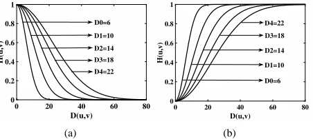
Fig. 2. Radial cross-section of (a) Lp-Gf and (b) Hp-Gf for different values of cut-offfrequency.
complexity of the frequency domain filtering is independent of the kernel size. More importantly, the proposed method uses
different cut-offfrequencies for Lp-gf and Hp-Gf, thus frequency domain filtering is preferred. Fig. 2(a) and (b) respectively show
the radial cross-sections of the Lp-Gf and Hp-Gf at different cut-offfrequencies used in the method. The proposed method analyses
AGKIs using Lp-Gf and Hp-Gf in frequency domain at different cut-offfrequencies. The Discrete Fourier Transform (DFT) of
an M×N AGKI I(x,y) is computed. The Fourier transformed AGKI, i.e., DFT (u,v) is translation invariant, but since it exhibits
the translational property of DFT, it is subjected to shift operation to ensure that the zero-frequency components are at the centre.
To represent the inner part of a silhouette gradually towards the centre more than its boundary, Lp-Gf is applied to the Fourier
transformed image using selected cut-offfrequencies, i.e.,
DFTL(u,v)=DFT (u,v)e(−(u
2+v2)/2D2)
, (4)
where e(−(u2+v2)/2D2)
is the transfer function of Lp-Gf [8], and DFTL(u,v) denotes the image filtered using Lp-Gf at the cut-off
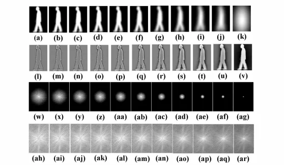
frequency D. The filtered AGKI at cut-offfrequency D in the image space is obtained by applying inverse DFT. Fig. 3(a)-(k) show
the AGKIs filtered by Lp-Gf with decreasing cut-offfrequency, and Fig. 3(w)-(ag) show the corresponding Fourier spectrum. Since
Lp-Gf attenuates high frequency components, it blurs the AGKI and smooths detailed clothing curvatures at its boundary. As the
cut-offfrequency decreases, it results in a greater loss of boundary and exterior regions (due to increase in blurring) to gradually
highlight the inner shape characteristics. Gaussian functions in the spatial and frequency domain behave reciprocally, hence an
increase in standard deviation of Lp-Gf in the spatial domain results in more blurring and vice versa [8].
To represent the boundary and exterior regions of an AGKI more than its central part, Hp-Gf is applied to the AGKI at the same
cut-offfrequencies, i.e.,
DFTH(u,v)=DFT (u,v)(1−e(−(u
2+v2)/2D2)
), (5)
where 1−e(−(u2+v2)/2D2) is the transfer function of Hp-Gf with cut-offfrequency D [8]. The filtered AGKI is similarly obtained
using inverse DFT. Fig. 3(l)-(v) shows the AGKIs filtered by Hp-Gf with decreasing cut-offfrequency and Fig. 3(ah)-(ar) show the
Fig. 3. Application of Lp-Gf (Row 1) and Hp-Gf (Row 2) to a AGKI from OU-ISIR dataset with decreasing cut-offfrequency: (a) & (l) D1=20; (b) & (m)
D2=18; (c) & (n) D3=16; (d) & (o) D4=14; (e) & (p) D5=12; (f) & (q) D6=10; (g) & (r) D7=8; (h) & (s) D8=6; (i) & (t) D9=4; (j) & (u) D10=3;
and (k) & (v) D11=1. Fourier spectrum at the corresponding cut-offfrequencies: row 3(Lp-Gf) and row 4 (Hp-Gf).
Fig. 4. (a) The original AGKI wearing (a) standard clothes and (l) down jacket from OU-ISIR gait dataset. The original AGKI (w) walking on grass without
a briefcase and (ah) walking on concrete with a briefcase from USF gait dataset. Application of Lp-Gf at at the cut-offfrequencies D1=20, D2=18, D3=
16, D4=14, D5=12, D6=10, D7=8, D8=6, D9=4, D10=3 on the AGKIs from OU-ISIR gait dataset (row 1 and 2) and USF gait dataset (row 3 and 4).
thus making the boundary characteristics of a silhouette more prominent, and its application represents the exterior regions of a
AGKI as the cut-offfrequency decreases. We used separable kernel to reduce the computational complexity of applying Gaussian
filters to an image of height h and width w to O(wkwh)+O(hkwh) as opposed to O(wkwhwh) for a non-separable kernel, where wk
and whrespectively denote the width and height of the kernel.
Fig. 4 demonstrates the robustness of the proposed method against variation in view and surface, and the presence of a carried
item with examples from two gait datasets, i.e., OU-ISIR gait dataset and USF HumanID gait dataset. Fig. 4(a)-(k) and (l)-(v)
respectively show the AGKI of a subject wearing standard clothes (type 9) (gallery) and the same subject with down jacket (probe)
from OU-ISIR gait dataset with their filtered versions using Lp-Gf at the cut-offfrequencies D1=20, D2=18, D1=16, D1=14,
D1=12, D1=10, D1=8, D1=6, D1=4, D1=3. Similarly, Fig. 4(w)-(ag) and (ah)-(ar) respectively show the AGKIs of a subject
walking on grass without a briefcase (gallery) and the same subject carrying a briefcase walking on a concrete surface (probe) from
[image:8.595.176.434.249.400.2]when respectively compared to Fig.3(a) and Fig.3(w), that the variation in clothing, carrying and surface cause significant shape
alterations at the boundary resulting in high intra-subject discrimination. The alteration decreases as the blurriness increases, and
disappears in the last column, where there is no difference between the gallery and its corresponding probe subject.
3.1.3. Cut-offfrequency selection
The cut-offfrequencies for Hp-Gf and Lp-Gf are selected based on focus value analysis of silhouettes. The focus value used
to measure the degree of sharpness of an image, is the maximum for the most focused, i.e., the original silhouette. It is inversely
proportional to the image blurriness caused by the Gaussian filtering at different cut-off frequencies. It has been graphically
demonstrated in [30] that the wavelet based method of computing focus value has the sharpest focus measure profile and higher
depth resolution compared to the spatial domain based methods, e.g., Tenengrad [25] and sum modified Laplacian [19], due to the
localised support property of wavelet basis. The first level 2D Daubechies-6 wavelet decomposition of a silhouette image f (x,y)
of size M×N results in four subband images, WLL, WHL, WLH and WHH, where L and H respectively denote lowpass filtered and
highpass filtered, and their order denotes the order of the filtering applied, e.g., WHL is a subband image obtained by highpass
filtering followed by lowpass filtering. The focus value (FV) of a silhouette is measured using [30]
FV= 1
MN
N
X
y=0
M
X
x=0
(|WHL(x,y)|+|WLH(x,y)|+|WHH(x,y)|). (6)
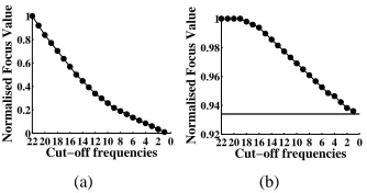
The focus value of the original silhouette always reduces to below 50% if it is filtered by Lp-Gf at cut-offfrequency D =
20, and decreases linearly as the blurriness increases with decreasing cut-offfrequencies. If the cut-offfrequency is decreased
further to below D=8, the focus value decreases abruptly. The focus value becomes infinitesimally small if D<4, resulting in
excessively blurred silhouette without any discriminating information (e.g., Fig. 3(j)-(k)). The boundary of a silhouette is obtained
by the application of Hp-Gf using D approximately in the range [18,22] for the USF dataset [22]. Since the silhouette boundary
corresponds to the sharpest image, e.g., Fig. 3(l)-(m), the focus value of a silhouette filtered by Hp-Gf using D in this range remains
the maximum which is considerably higher than the focus value of the original silhouette (i.e., Fig. 5(b)). With further decrease
in cut-offfrequency, the focus value decreases linearly with a decrease in sharpness of the image as the silhouette is reconstructed
by regaining its central region. The focus value is nearly identical to that of the focus value of the original silhouette in the range
1≤D<4 due to almost perfect reconstruction of the original silhouette. Since the boundary as well as central shape characteristics
of a silhouette are considered separately by using Lp-Gf and Hp-Gf, it is not necessary to use cut-offfrequencies in the range
1≤D<4 which will increase the computational complexity. Thus, [4,20] is considered to be the ideal range of cut-offfrequencies.
Fig. 5 (a) and (b) respectively show the normalised focus value w.r.t. decreasing cut-offfrequencies in the range [22,0] of a
0 2 4 6 8 10 12 14 16 18 20 22 0 0.2 0.4 0.6 0.8 1 Cut−off frequencies
Normalised Focus Value
(a) 0 2 4 6 8 10 12 14 16 18 20 22 0.92 0.94 0.96 0.98 1 Cut−off frequencies
Normalised Focus Value
[image:10.595.220.387.39.127.2](b)
Fig. 5. Normalised focus value w.r.t. decreasing cut-offfrequencies of a silhouette from USF 2.1 dataset filtered using (a) Lp-Gf; and (b) Hp-Gf. ’-’ denotes
focus value of the original silhouette.
focus value in the range [22,0]. Fig. 5 shows the focus value of a filtered silhouette maintains an almost linear relationship with the
cut-offfrequencies of the Gaussian filters.
The identification rate of a gait recognition method increases if the discriminability between the different subjects is high, while
the same subject shows similar shape characteristics despite variation in clothing and carrying conditions in different situations.
Also, the computational complexity is directly proportional to the the number of cut-offfrequencies. Hence, we chose the minimum
three cut-offfrequencies based on the following three cases. For case 1, the discriminability between different subjects with no
variation in clothing and carrying conditions is high: least blurring (for Lp-Gf) and accurate boundary (for Hp-Gf) are desirable to
satisfy this. Thus, the upper cut-offof the ideal range of cut-offfrequencies, i.e., D=20 for both Lp-Gf and Hp-Gf is selected. For
case 2, i.e., same subjects with small shape distortions due to variation in carrying conditions, hair style and presence of shadows
under feet show similar shape characteristics: medium blurring and considerably regained central region of the AGKI are desirable.
Hence, the mid value of the ideal range of cut-offfrequency, (i.e., D=12) for lp-Gf and lower cut-offfrequency for Hp-Gf, (i.e.,
D=4) are chosen. For case 3, the drastic shape variation of the same subject due to unpredictable variation in clothing is taken
into account. Thus, the cut-offfrequency which causes excessive blurring for Lp-Gf, i.e., the lower bound of the ideal range of
cut-offfrequencies, i.e, D=4 is chosen. For Hp-Gf, this requires midway of the prominent boundary and almost reconstruction of
the original silhouette, hence, D=12 is appropriate. Thus, the three cut-offfrequencies chosen for Lp-Gf and Hp-Gf are 4, 12 and
20. In view of this experimental analysis, the following inferences are made for any dataset:
• 1: The cut-offfrequency for Lp-Gf at which the focus value of the original silhouette always reduces to below 50% can be
used for Hp-Gf to obtain the boundary of the silhouette. This frequency is chosen as the upper-bound of the ideal range of
the cut-offfrequencies.
• 2: The cut-offfrequency for Lp-Gf below which the focus value becomes infinitesimally small can be used as the cut-off
frequency for Hp-Gf at which the silhouette is perfectly reconstructed. This frequency is chosen as the lower-bound of the
ideal range of cut-offfrequencies.
mid-value are used.
3.2. Module 2: subject classification using rotation forest
3.2.1. Training
Let x = [x1, ...,xn]T be a gallery subject described by n features, where n=30 corresponds to the five AGKIs filtered using
Lp-Gf and Hp-Gf, each at 3 cut-offfrequencies (i.e., 5×3+3=30), and N be the total number of subjects in the gallery. The gallery
dataset, i.e., X, is thus represented by N×n matrix. Let Y=[y1, ...,yN]Tbe the class labels{1,...,c}for the dataset, and c be the
total number of gallery classes of subjects. Let D1, ..., DLdenote the classifiers in the ensemble, and F, the feature set. The steps to
train the classifier Difor i=1,...,L are:
• F is randomly split into K disjoint subsets, and each subset contains M=n/K features.
• Let Fi,jbe the jth subset of features for Dicontaining Xi,jfeatures from X, where j=1,...,K. A new training set, i.e., Xi′,j,
is selected from Xi,jrandomly with 75% size using bootstrap algorithim. Xi′,jis subjected to principal component analysis
(PCA) to obtain the principal components, i.e., a(1)i,j,..., a(Mj)
i,j each of size M×1. PCA is used as the transformation algorithm
due to its superiority to independent component analysis, maximum noise fraction and local Fisher discriminant analysis for
the case of rotation forest ensemble classifier, as experimentally demonstrated in [28].
• The coefficients are organised in a sparse rotation matrix Riof dimensionality n×PjMjas follows:
Ri=
a(1)i,1, ...,a(M1)
i,1 0 · · · 0
0 a(1)i,2, ...,a(M2)
i,2 · · · 0
..
. ... . .. ...
0 0 · · · a(1)i,K, ...,a(MK)
i,K
The columns of Riare rearranged to Rai with respect to the original feature set to construct the training set XRai for the classifier
Di.
3.2.2. Classification
For a given test sample x, let di,j(xRai) be the probability assigned by the classifier Dithat x belongs to class wj. The confidence
for each class, i.e., wj, is calculated by the average combination method as
µj(x)=
1 L
L X
i=1
di,j(xRai),j=1, ...,c, (7)
where L is the ensemble size. x is assigned to the class with the largest confidence. The percentage of correct classification rate is
CCR=sc/st∗100, where scand stare respectively the number of correctly identified subjects and the total number of subjects in
the dataset. To increase the statistical significance of the results, CCR is obtained as the average of 10 runs for specified values of
values with their matching gallery classes. Thus, CCR at rank-1 implies that the probe subjects result in the highest confidence
values with their matching gallery classes, similarly CCR at rank-5 implies that the correctly identified probe subjects are within
the top 5 highest confidence values.
3.2.3. Sensitivity of Parameters
The key parameters of rotation forest are L and M. Since the aim of the paper is to demonstrate the efficacy of the application of
Gaussian filtering at multiple cut-offfrequencies to achieve robustness to unpredictable variation in clothing and carrying conditions
rather than achieve higher W-AvgI through intensive parameter calibration, we fix M=5 for all values of L used in the proposed
method, as very high value of M causes overlearning.
4. Experiments
The proposed method is evaluated using two public datasets: USF HumanID gait challenge dataset [22] and OU-ISIR treadmill
gait dataset B [18].
The HumanID gait challenge problem in [22] has three aspects: a dataset, 12 challenge experiments and a baseline algorithm.
The large version of USF HumanID gait challenge dataset comprises 1870 sequences of 122 subjects walking along an elliptical
path in an outdoor environment in front of two cameras. The dataset provides up to 32 possible testing conditions by combining
the following five covariates: (a) walking surface (grass (G) or concrete (C)); (b) shoe type (A or B); (c) viewpoint (right (R) or
left (L)); (d) carrying conditions (carrying a briefcase (BF) or not carrying a briefcase (NB)); and (e) elapsed time between the
acquisition of the sequences (May (M) or November (N)). The 12 challenge experiments, i.e., probe sets (A to L), are designed for
investigating the effects of five covariates on gait recognition. The structure of the probe sets as standardized in [22] is shown in
Table 1. All probe sets do not contain the same number of subjects, and there are no common gait sequences between the gallery
set and any of the probe sets.
The dataset provides centre-aligned and scale-normalised silhouettes of fixed size 128×88 which could be downloaded from
http://figment.csee.usf.edu/GaitBaseline/. As explained in the baseline algorithm, the silhouette bounding boxes of the first, last
and the middle frames of a gait sequence are computed manually, and the bounding boxes of the intermediate frames are generated
using linear interpolation. After the semi-automated process of bounding box estimation, the iterative expectation-maximisation
process of background subtraction is used to extract the foreground, i.e., the silhouette. The silhouette is normalised to a height of
128 pixels, and centralised by coinciding its centre-of-mass with the centre of the frame.
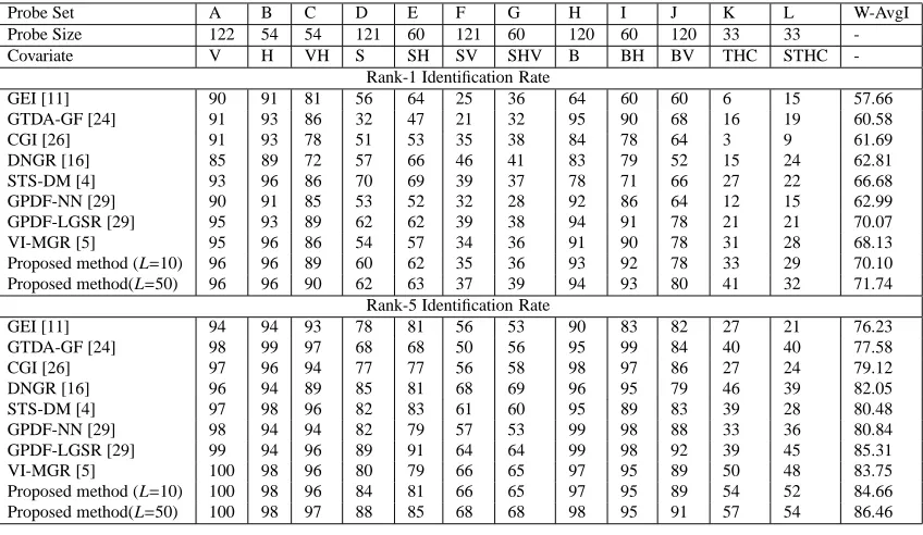
Table 1 shows the classification rates of the proposed method using L=10, 50 at ranks 1 and 5 for comparison with the
state-of-the-art methods that outperform Baseline on the USF dataset. All methods in Table 1 use the same gallery set (G, A, R, NB,
Table 1. Classification rates (%) at rank-1 and rank-5 of the gait recognition methods on full version of USF HumanID gait challenge dataset using the gallery set (G, A, R, NB, M/N) of 122 subjects. Keys for covariates: V - view; H - shoe; S - surface; B - briefcase; T - time; and C - clothes.
Probe Set A B C D E F G H I J K L W-AvgI
Probe Size 122 54 54 121 60 121 60 120 60 120 33 33
-Covariate V H VH S SH SV SHV B BH BV THC STHC
-Rank-1 Identification Rate
GEI [11] 90 91 81 56 64 25 36 64 60 60 6 15 57.66
GTDA-GF [24] 91 93 86 32 47 21 32 95 90 68 16 19 60.58
CGI [26] 91 93 78 51 53 35 38 84 78 64 3 9 61.69
DNGR [16] 85 89 72 57 66 46 41 83 79 52 15 24 62.81
STS-DM [4] 93 96 86 70 69 39 37 78 71 66 27 22 66.68
GPDF-NN [29] 90 91 85 53 52 32 28 92 86 64 12 15 62.99
GPDF-LGSR [29] 95 93 89 62 62 39 38 94 91 78 21 21 70.07
VI-MGR [5] 95 96 86 54 57 34 36 91 90 78 31 28 68.13
Proposed method (L=10) 96 96 89 60 62 35 36 93 92 78 33 29 70.10
Proposed method(L=50) 96 96 90 62 63 37 39 94 93 80 41 32 71.74
Rank-5 Identification Rate
GEI [11] 94 94 93 78 81 56 53 90 83 82 27 21 76.23
GTDA-GF [24] 98 99 97 68 68 50 56 95 99 84 40 40 77.58
CGI [26] 97 96 94 77 77 56 58 98 97 86 27 24 79.12
DNGR [16] 96 94 89 85 81 68 69 96 95 79 46 39 82.05
STS-DM [4] 97 98 96 82 83 61 60 95 89 83 39 28 80.48
GPDF-NN [29] 98 94 94 82 79 57 53 99 98 88 33 36 80.84
GPDF-LGSR [29] 99 94 96 89 91 64 64 99 98 92 39 45 85.31
VI-MGR [5] 100 98 96 80 79 66 65 97 95 89 50 48 83.75
Proposed method (L=10) 100 98 96 84 81 66 65 97 95 89 54 52 84.66
Proposed method(L=50) 100 98 97 88 85 68 68 98 95 91 57 54 86.46
Table 1). Since there are different number of probe subjects in the challenge experiments, the weighted average classification rate
(W-AvgI) is obtained using [4, 29]
W-AvgI=
Pg
i=1wixi Pg
i=1wi
, (8)
where g denotes the number of challenge experiments, i.e., 12, for Exp. A-L, xidenotes the CCR of the ith challenge experiment
and widenotes the number of probe subjects participating in that experiment. Table 1 shows the final W-AvgI of VI-MGR computed
by averaging the identification rates obtained by weighted random subspace learning for eighty randomly chosen values of number
of subspaces in the range [100,500]. The table shows that our method achieves W-AvgI)=71.74% at rank-1 and 86.46% at rank-5
for L=50, thus outperforming all other methods. The performance of our method is analyzed using cumulative match characteristic
(CMC) curve for the 12 challenge experiments (see Fig. 6(a)). According to this curve, W-AvgI at rank r implies that the percentage
of correctly identified subjects is among the top r largest confidence values.
4.1. OU-ISIR Treadmill Gait Dataset
The OU-ISIR gait dataset [18] consists of four components, i.e., dataset A, dataset B, dataset C and dataset D to respectively
facilitate the evaluation of gait recognition methods in the presence of variations in speed, clothing, view, and gait fluctuation. Our
method is evaluated on the dataset B which comprises 68 subjects with up to 32 combinations of different types of clothing. Table 2
shows these clothing combinations based on the 15 different types of clothes used in constructing the dataset [13]. The dataset
Table 2. Different clothing combinations used in the OU-ISIR B dataset. Keys for different types of clothes: RP-Regular pants; BP-Baggy pants; SP-Short pants; Sk-Skirt; CP: Casual pants; HS-Half shirt; FS- Full shirt; LC-Long coat; Pk-Parker; DJ-Down jacket; CW-Casual wear; RC-Rain coat; Ht-Hat; Cs-Casquette cap; Mf-Muffler.
Type S1 S2 S3 Type S1 S2 Type S1 S2
3 RP HS Ht 0 CP CW F CP FS
4 RP HS Cs 2 RP HS G CP Pk
6 RP LC Mf 5 RP LC H CP DJ
7 RP LC Ht 9 RP FS I BP HS
8 RP LC Cs A RP Pk J BP LC
C RP DJ Mf B RP Dj K BP FS
X RP FS Ht D CP HS L BP Pk
Y RP FS Cs E CP LC M BP DJ
N SP HS - P SP Pk R RC
-S Sk HS - T Sk FS U Sk PK
V Sk DJ - Z SP FS - -
-Rank
0 5 10 15 20
W-AvgI
20 40 60 80 100
(a)
Probe Clothing Combination
0 2 3 4 5 6 7 8 9ABCDEFGH I JKLMNPRSTUVXYZ
Rank-1 Classification Rate (%)
0 20 40 60 80 100
VI-MGR Proposed Method GEI
(b)
Fig. 6. (a) Performance analysis using CMC curve on 12 challenge experiments of USF gait data set. Keys: ’✄’- Exp. A (Probe: G, A, L, NB, M/N); ’✸
’-Exp. B (Probe: G, B, R, NB, M/N); ’×’- Exp. C (Probe: G, B, L, NB, M/N); ’✷’- Exp. D (Probe: C, A, R, NB, M/N); ’⋆’- Exp. E (Probe: C, B, R, NB,
M/N); ’•’- Exp. F (Probe: C, A, L, NB, M/N); ’△’- Exp. G (Probe: C, B, L, NB, M/N); ’∗’- Exp. H (Probe: G, A, R, BF, M/N); ’◦’- Exp. I (Probe: G, B,
R, BF, M/N); ’_’- Exp. J (Probe: G, A, L, BF, M/N); ’’- Exp. K (Probe: G, A/B, R, NB, N); and ’▽’- Exp. L (Probe: C, A/B, R, NB, N); (b) Rank 1
classification rate for 32 probe items of OU-ISIR dataset B with different clothing combinations using gallery set of subjects with RP+FS.
set comprising 446 sequences of 20 subjects with all types of clothes; (b) a gallery set comprising sequences of the remaining 48
subjects with standard clothes (type 9); and (c) a probe set comprising 856 sequences for these 48 subjects with other types of
clothes excluding the standard clothes.
Unlike the method in [13], the goal of our method is to demonstrate robustness against unpredictable variation in clothing.
Hence, unlike [13], we do not use the training dataset to train our system with all possible types of clothing combinations. We
evaluated GEI on OU-ISIR dataset B using gallery and probe sets each comprising 48 subjects to compare with the proposed
method. Fig. 6(b) shows the results of comparisons with GEI and VI-MGR (available from [5]). The figure shows that our method
significantly outperforms GEI and VI-MGR at rank-1 CCR.
5. Conclusion and future work
The paper introduces a gait representation, AGKI, by averaging each of the five key frames of a gait period over a gait sequence.
The AGKIs are subjected to Lp-Gf and Hp-Gf at different cut-offfrequencies to achieve invariance to unpredictable variation in
[image:14.595.182.429.85.341.2]Experimental analyses on two public datasets demonstrate the efficacy of the method.
Future studies will include: (a) taking into consideration of view-invariant gait characteristics while forming AGKI to achieve
robustness to variation in view by developing a view transformation model; (b) detailed experimental analyses on the choice of L
and M to achieve improved identification rate.
References
[1] Bashir, K., Xiang, T., Gong, S., 2010. Gait recognition without subject cooperation. Pattern Recognition Letters 31, 2052–2060. [2] Breiman, L., 1996. Bagging predictors. Machine Learning 24, 123–140.
[3] Choudhury, S.D., Tjahjadi, T., 2012. Silhouette-based gait recognition using procrustes shape analysis and elliptic fourier descriptors. Pattern Recognition 45, 3414–3426.
[4] Choudhury, S.D., Tjahjadi, T., 2013. Gait recognition based on shape and motion analysis of silhouette contours. Computer Vision and Image Understanding 117, 1770–1785.
[5] Choudhury, S.D., Tjahjadi, T., 2015. Robust view-invariant multiscale gait recognition. Pattern Recognition 48, 798–811.
[6] Freund, Y., Schapire, R., 1997. A decision-theoretic generalization of on-line learning and an application to boosting. Journal of Computer and System Sciences 55, 119–139.
[7] G. Bradski, A.K., 2008. Learning OpenCV Computer Vision with the OpenCV Library. 1st ed., O’Reilly Media, Sebastopol. [8] Gonzalez, R.C., Woods, R.E., 1992. Digital image processing. 2nd ed., Addison-Wesley, USA.
[9] Gu, J., Ding, X., Wang, S., Wu, Y., 2010. Action and gait recognition from recovered 3-d human joints. IEEE Transactions on Systems, Man and Cybernetics, Part B: Cybernetics 40, 1021–1033.
[10] Guan, Y., Li, C.T., Hu, Y., 2012. Random subspace method for gait recognition. in: Proceedings of the IEEE International Conference on Multimedia and Expo Workshop (ICMEW’12) , 9–13.
[11] Han, J., Bhanu, B., 2006. Individual recognition using gait energy image. IEEE Transactions on Pattern Analysis and Machine Intelligence 28, 316–322. [12] Ho, T.K., 1998. The random subspace method for constructing decision forests. IEEE Transactions on Pattern Analysis and Machine Intelligence 20, 832–844. [13] Hossain, M.A., Makihara, Y., Wang, J., Yagi, Y., 2010. Clothing-invariant gait identification using part-based clothing categorization and adaptive weight
control. Pattern Recognition 43, 2281–2291.
[14] Ioannidis, D., Tzovaras, D., Damousis, I.G., Argyropoulos, S., Moustakas, K., 2007. Gait recognition using compact feature extraction transforms and depth information. IEEE Transactions on Information Forensics and Security 2, 623–630.
[15] Lam, T.H.W., Cheung, K.H., Liu, J.N.K., 2011. Gait flow image: A silhouette-based gait representation for human identification. Pattern Recognition 44, 973–987.
[16] Liu, Z., Sarkar, S., 2006. Improved gait recognition by gait dynamics normalization. IEEE Transactions on Pattern Analysis and Machine Intelligence 28, 863–876.
[17] Lu, H., Plataniotis, K.N., Venetsanopoulos, A.N., 2008. A full-body layered deformable model for automatic model-based gait recognition. EURASIP Journal on Advances in Signal Processing , 1–13.
[18] Makihara, Y., Mannami, H., Tsuji, A., Hossain, M.A., Sugiura, K., Mori, A., Yagi, Y., 2012. The ou-isir gait database comprising the treadmill dataset. IPSJ Transactions on Computer Vision and Applications, Technical Note 4, 53–62.
[19] Nayar, S.K., Nakagawa, Y., 1994. Shape from focus. IEEE Transactions on Pattern Analysis and Machine Intelligence 16, 824–831.
[20] Ran, Y., Zheng, Q., Chellappa, R., Strat, T.M., 2010. Applications of a simple characterization of human gait in surveillance. IEEE Transactions on Systems, Man, and Cybernetics, Part B: Cybernetics 40, 1009–1019.
[21] Rodrguez, J.J., Kuncheva, L.I., Alonso, C.J., 2006. Rotation forest: A new classifier ensemble method. IEEE Transactions on Pattern Analysis and Machine Intelligence 28, 1619–1630.
[22] Sarkar, S., Philips, P.J., Liu, Z., Vega, I., Grother, P., Bowyer, K., 2006. The humanid gait challenge problem: data sets, performance, and analysis. IEEE Transactions on Pattern Analysis and Machine Intelligence 27, 162–177.
[23] Tafazzoli, F., Safabakhsh, R., 2010. Model-based human gait recognition using leg and arm movements. Engineering Applications of Artificial Intelligence 23, 1237–1246.
[24] Tao, D., Li, X., Wu, X., Maybank, S.J., 2007. General tensor discriminant analysis and gabor features for gait recognition. IEEE Transactions on Pattern Analysis and Machine Intelligence 29, 1700–1715.
[25] Tenenbaum, J.M., 1970. Accommodation in computer vision. Ph.D. Thesis , Stanford University.
[26] Wang, C., Zhang, J., Wang, L., Pu, J., Yuan, X., 2012. Human identification using temporal information preserving gait template. IEEE Transactions on Pattern Analysis and Machine Intelligence 34, 2164–2176.
[27] Wang, L., Tan, T., Ning, H., Hu, W., 2003. Silhouette analysis-based gait recognition for human identification. IEEE Transactions on Pattern Analysis and Machine Intelligence 25, 1505–1518.
[28] Xia, J., Du, P., He, X., Chanussot, J., 2014. Hyperspectral remote sensing image classification based on rotation forest. IEEE Geoscience and Remote Sensing letters 11, 239–243.
[29] Xu, D., Huang, Y., Zeng, Z., Xu, X., 2012. Human gait recognition using patch distribution feature and locality-constrained group sparse representation. IEEE Transactions on Image Processing 21, 316–326.