Atomistic to continuum coupling

(1)

warwick.ac.uk/lib-publications

A Thesis Submitted for the Degree of PhD at the University of Warwick

Permanent WRAP URL:

http://wrap.warwick.ac.uk/101783

Copyright and reuse:

This thesis is made available online and is protected by original copyright.

Please scroll down to view the document itself.

Please refer to the repository record for this item for information to help you to cite it.

Our policy information is available from the repository home page.

(2)

M A

O

D

C

S

Atomistic-to-continuum coupling

by

Huan Wu

Thesis

Submitted for the degree of

Doctor of Philosophy

Mathematics Institute

The University of Warwick

(3)

Acknowledgments

It has been eight years for me at the University of Warwick, including my undergraduate

study. The Warwick Mathematics Institute has become a second home to me. I immensely

appreciate the supporting and encouraging environment that WMI has provided during

my time here.

Most importantly, I would like to address a special thanks to my First Supervisor

Professor Christoph Ortner and Second Supervisor Professor Andreas Dedner, who have

generously put their experience and wisdom at my disposal. In particular, I would like to

express my enormous gratitude to Professor Christoph Ortner who I have worked closely

for four years and has inspired me beyond academics with his incredible intelligence and

work ethic.

I would also like to thank Professor Charlie Elliott, who was my undergraduate

tutor and continued his support during my postgraduate study.

The Mathematics and Statics Centre for Doctoral Training has provided excellent

research environment and I would like to thank the staff of this centre. My funding body

Engineering and Physical Sciences Research Council has provided financial support to me.

I should also mention my MASDOC colleagues: Faizan, Simon, Ben, Jere, Jorge,

Graham, David, Ollie, Matt, Jack, John, Jake, Jamie and Luke, who not only shared their

wisdom but also contributed to many happy memories during my life at Warwick. I would

also like to thank my friends Becky, Fei, Anna and Orange who accompanied me through

difficulties.

Last but not least I would like to thank my parents Lifang Guo and Bin Wu. I

(7)

Declarations

I declare that this thesis is the result of my own work, except where otherwise stated. I

declare that any part of this thesis has not previously been submitted for a degree or any

other qualification at this University or any other institution. I declare that Chapter 3

has been accepted by ESAIM: Mathematical Modelling and Numerical Analysis (ESAIM:

M2AN) and published on https://arxiv.org/abs/1607.05936 with title “Analysis of

patch-test consistent atomistic-to-continuum coupling with higher-order finite elements”.

I declare that Chapter 4 has been published onhttp://arxiv.org/abs/1709.05977with

(8)

Abstract

The present thesis is on error analysis of atomistic-to-continuum (A/C) coupling models

for crystal defects, which is a class of multi-scale coupling models that combine atomistic

interactions around the defect cores and continuum elasticity models at far-fields.

This thesis consists of two parts. The first part presents a sharp error analysis of an

A/C model in 2D with high-order finite element methods, whereas in the past the analysis

for employing FEM has been restricted to first-order. The second part discusses a new

A/C coupling scheme employing a boundary element method to improve the description

of the far-field.

In the first part we formulate a “patch test consistent” atomistic-to-continuum

coupling (a/c) scheme that employs a second-order (potentially higher-order) finite element

method in the material bulk. We prove a sharp error estimate in the energy-norm, which

demonstrates that this scheme is (quasi-)optimal amongst energy-based sharp-interface

a/c schemes that employ the Cauchy–Born continuum model. Our analysis also shows

that employing a continuum discretization with order greater than two does not yield

qualitative improvements to the rate of convergence.

In the second part we formulate a new A/C coupling scheme that employs a

bound-ary element method to obtain an improved far-field boundbound-ary condition. We establish

sharp error bounds in a 2D model problem for a point defect embedded in a homogeneous

crystal. The error analysis shows that it is possible to entirely bypass the FEM region

while maintaining an optimal convergence rate.

The thesis is accompanied by an introduction to atomistic-to-continuum coupling

and literature review on various coupling methods and the general framework for error

(9)

Chapter 1 Introduction

Material science has become increasingly prominent over the past several decades, in part

due to advances in molecular modeling and new engineering tools. The study of nanoscale

systems opens up opportunities in a wide range of applications, including medical diag-nostic, material reinforcement, chemical sensing, material design and so on. Once the

physical models for materials are established, computational methods are developed.

De-spite the rapid development of computing powers, simulations on full microscopic scale are still too costly. This is due to the fact that many materials display different properties at

different length and time scales. For example, the strengthening properties of steel exist

at different material length scales, ranging from quantum scale with atomic lattice uncer-tainties, to submicroscale with thermodynamics unceruncer-tainties, to microscale inclusions, to

ultimately macroscale of the formation of a ship (see Figure 1.1 ). Single-scale models are

not sufficient for this type of systems.

Multiscale coupling is a class of modeling methods that describe microscopic

config-urations of regions of interest, and approximate using coarser models (such as continuum

mechanics) far away from the “core areas”. In principle these methods can reduce com-putational costs while maintaining the accuracy of the atomistic models.

At the defect core, the material displays atomistic behaviours that cannot be eled by macroscopic systems. But outside the defect core, the elastic fields are often

mod-eled by continuum mechanics. The resulted techniques are called atomistic-to-continuum

coupling (a/c) methods. They are a prototypical atomistic-level multi-scale scheme. Us-ing finite element schemes on a coarse mesh in the continuum region further improves

computational efficiency.

Early ideas of a/c coupling occurred in several works from 1950s to 1970s, such as [26] and [50] using continuum linear elasticity to describe far-field behaviour. Later

on the methodology of employing finite elements to discretize the continuum model was

introduced in [37], [19] and [27]. The introduction of variational framework and the Cauchy–Born model by [38] was a key step for the development of a/c coupling. Since

then the term “quasicontinuum” is widely used. It is now widely understood that the

(10)

[image:10.595.124.481.92.314.2]

Figure 1.1: Multiscale properties of steel. This illustration is taken from [31]

methods have been proposed: the quasi-non-local coupling [49], blending schemes [55], force-based a/c coupling [36], and the ghost force correction method [48]. In Chapter 2,

we briefly introduce the concepts of blending type methods and ghost forces. Throughout

this thesis we focus on quasi-non-local (QNL) coupling and the error analysis resulting from both the coupling method and the use of different numerical schemes for describing

bulk elasticity.

In terms of numerical simulations, it is important to quantify the accuracy of the simulation to determine how good the models and numerical schemes are. The continuum

regions of a/c coupling methods are usually computed on coarse meshes in order to reduce

cost. On the other hand, it is crucial to ensure that the numerical schemes do not add significant inaccuracy to the simulation. So it is necessary to balance these two aspects

to obtain optimal computational parameters. Thus our goal is to determine the

“opti-mal error” that can be obtained from numerical simulations with a given computational cost. This involves both analysis of the pure modelling error of non-linear coupled

sys-tems and error estimation and optimization of finite element schemes and other optimal

(11)

Chapter 2 Background

2.1 Interatomic potentials

In this section, we introduce interatomic potentials for crystals. Let Z be an index set.

The (deformed) atom configuration is represented by y : Z _→ Rd, d= 1,2,3. Then the

distance between two atom positions is written asRij :=|y(i)−y(j)|.

2.1.1 Pair potentials

Pair potentials are the simplest interatomic potentials. For a configuration y : Z _→ Rd,

d= 1,2,3, the potential energy is written as

E(y) = X

i,j∈Z,i6=j

φ(_|y(i)₋y(j)_|),

whereφ : [0,_∞) _→ R∪ {+∞}is a pair potential. The Lennard-Jones potential ([25]) is

an example which is widely used in molecular simulations. It is given by

φLJ(r) :=r−12−2r−6.

2.1.2 The embedded atom method (EAM)

Phenomenological observations of metallic systems indicate the presence of significant many-atom interactions which pair potential models fail to describe. Table 1 in [11] shows

that Ni, Cu, Pd, Ag, Pt and Au all display many-body effects. Consequently there is a

need for more complex models that capture the fact that, in general, bond interactions are not independent from each other.

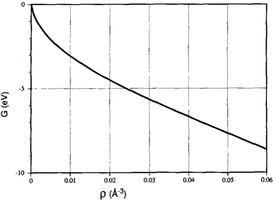
In [10] the embedded atom method was proposed, in which the total energy is

obtained by embedding an atom into the local electron density provided by the rest of the atoms in the system, in addition to an electrostatic interaction. The general formulation

(12)

[image:12.595.163.440.87.288.2]

Figure 2.1: Embedding energy of Ni as a function of the density of background electron gas. This figure is copied from [11].

E(y) =X

i∈Z

E_iEAM(y), (2.1.1)

with

E_iEAM(y) :=G

 

X

j∈Z,j6=i

ρj(Rij)

 +

X

j∈Z,i6=j

φ(Rij),

where G is the embedding energy, ρj is the atomistic electron density, the summation

P

j∈Z,j6=iρj(Rij) represents the spherically averaged electron density andφis the

electro-static two-atom interaction. The embedding energyGis defined by the interaction of the atom with the background electron gas. Figure 2.1 is an example of an embedding energy.

The background densityρ is determined by evaluating at its nucleus the superposition of

atomic-density tails from the other atoms. Figure 2.2 is an example of pair interaction. As we can see from the formulation, EAM is inherently more complex than

pair-bond models.

2.1.3 General site energies

All interatomic potential energies can be written in the form of site energies, namely, for

an atom position mapy:Z _→Rd,

E(y) =X

`∈Z E`(y),

whereE`(y) are the site energies.

For the sake of analysis, we need the following assumptions onE`:

(13)

[image:13.595.165.439.83.286.2]

Figure 2.2: Pair interaction of Ni as a function of separation. This figure is copied from [11].

E`(y).

2. Permutation invariance: for all permutations p of Z, and yp(`) := y(p(`)), we

have Ep(`)(y) =E`(yp).

3. Smoothness: E` is a “smooth” function of y for the “required range” of

configu-rations y. Normally, we require that E` is smooth at all configurationsy for which y` 6=yn for all `, n∈Z.

4. Locality: there existsrcut>0 such thatE` is only a function of |y`−yk|< rcut.

2.2 Crystals and defects

2.2.1 Lattices

In the present work, we are concerned with crystalline solids, described in the form of

Bravais lattices.

Definition 2.2.1. A Bravais lattice is defined by AZd with d= 1,2,3, where A∈Rd×d

is non-singular. For example, in Chapter 2, we discuss a triangular lattice in 2D with

A= 1 cos(π/3)

0 sin(π/3)

!

.

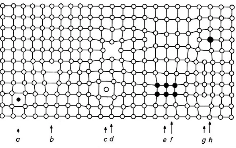
2.2.2 Point defects

In reality, atoms in solids are not arranged in perfect lattices. One of the reasons causing

(14)

[image:14.595.111.489.98.335.2]

Figure 2.3: a) Interstitial impurity atom, b) Edge dislocation, c) Self interstitial atom, d) Vacancy, e) Precipitate of impurity atoms, f) Vacancy type dislocation loop, g) Inter-stitial type dislocation loop, h) Substitutional impurity atom. This illustration is drawn by Helmut F¨oll and is taken fromhttps://www.tf.uni-kiel.de/matwis/amat/def_en/ overview_main.html

In the present work, we focus on point defects. Examples include impurities,

in-terstitials and vacancies (a, c and d in Figure 2.3 respectively).

To simulate point defect configurations, we first set up a reference configuration

Λ_⊂Rdthat coincides with a Bravais lattice far away from the defect core.

Definition 2.2.2. [18] A discrete set Λ is a point defect reference configuration if there exists a Bravais latticeΛhom and a radius Rcore such that Λ\BRcore = Λ

hom_\_B

Rcore and

Λ_∩BRcore is finite.

2.2.3 Dislocations

Dislocations have been intensively studied since they are the carriers of plastic deformation.

Generally speaking there are two types of dislocations:

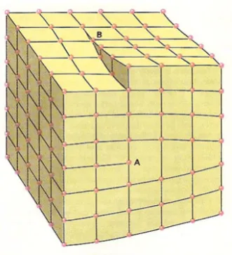
1. Edge dislocations: produced by a half-plane inserted or removed from the lattice,

see b) and g) in Figure 2.3 and A in Figure 2.4.

2. Screw dislocations: created by slip parallel to the dislocation line, see B in Figure

2.4.

(15)

[image:15.595.216.382.84.266.2]

Figure 2.4: Section of a crystal lattice including an edge dislocation (A) and a screw dislocation (B). This illustration is drawn by David Darling and is taken from http: //www.daviddarling.info/encyclopedia/D/dislocation.html.

numerical discretization aspects rather than atomistic mechanics aspects, later chapters

of this thesis will be restricted to point defect only.

2.3 Atomistic-to-continuum models

The first key step in a/c multi-scale modelling is to approximate the atomistic model by a continuum elasticity model. In this way we can reduce the computational costs while

maintaining significant accuracy. One of the mostly widely used continuum models is the

Cauchy–Born model, which will be used throughout this thesis.

2.3.1 The Cauchy–Born model

The Cauchy–Born model introduced by [6] and [4] has been widely employed as the

con-tinuum model in a/c coupling. The Cauchy–Born potential is an elastic potential derived

from the atomistic energy by averaging the energy per unit volume. It is a useful tool for macroscopic models since the elastic response is derived from the interatomic

poten-tial without the need for fitting parameters. Various a/c coupling methods have been developed based on the Cauchy–Born model.

For a homogeneous configuration Λ = AZd, The physical position of a defective

lattice is described by a deformation map y : Λ → Rd. Define the displacement map

u: Λ_→Rdasu:=y−x. Let us consider an atomistic energy with interaction range Rnn.

Long-range interactions (i.e. interaction range greater thanRnn) can be treated using the

same approach. The atomistic energy is then given by

Ehom₍_u_{) =}X

`∈Λ

(16)

where

Du(`) =u(`)₋u(k)

|`−k|<Rnn,`6=k

.

Formally we can rescale space and energy by Λ Λ, x x,u u, and V d_V _for >0. The scaled energy is written as

Ehom (u) =

X

`∈Λ

dV(Du(`)),

where

Du(`) :=

u(`)₋u(k)

|`−k|<Rnn,`6=k

.

Letting_→0 gives the Cauchy–Born energy [24]

Ehom→ Ec:=

Z

Rd

W(_∇u˜)dx,

where

W(F) :=V(Fξ)_{ξ∈Λ\0,|ξ|<R}_nn, F_∈Rd×d,

˜

uis some continuous interpolant of u. In later sections we will discuss the formulation of the Cauchy–Born strain energy functionW :Rd×d→Rfor specific models.

2.3.2 Quasicontinuum coupling

To incorporate atomistic models around defects with elastic continuum models at far-field, quasicontinuum (QC) coupling has been proposed in [38]. The original QC coupling is

rather intuitive. Formally, the fully atomistic energy in terms of each atom is written as

Ea₌X

`∈Λ E_`a.

Outside the defect bulk, the energy can be approximated by a continuum model with

appropriate elasticity strain derived from the atomistic interactions. Formally, the (local) continuum energy at each atom` is written as

E_`c=

Z

ω`

W(_∇u)

whereω`are non-overlapping regions containing one atom only. Throughout this thesis we

employ the Cauchy–Born potential as the elasticity strain energy. Such atoms are called

local because the energy is irrelevant to the atoms outside the element. See_§2.4, _§3.1 for

specific examples ofEa _and _Ec_{in 1D and 2D respectively. The quasicountinuum coupling}

energy is then given by

Eac=X

`∈A

E_`a+X

`∈C

E_`c, (2.3.1)

(17)

ghost forces

A

C

[image:17.595.126.468.80.173.2]

local interaction

Figure 2.5: Ghost forces from a QC model on a homogenenous lattice in 1D. We assume next-nearest-neighbour interaction in the atomistic region _A, whereas the Cauchy–Born energy in the continuum region is local.

However, as demonstrated in [49], the QC energy formulation above results in non-zero forces around the interface atoms, which areghost forces. This is formally explained

as follows.

Letu be a homogeneous displacement on a lattice Λ⊂Rd, i.e. u(x) :=F·x, where

F_∈Rd×d . The ghost force on each atom`∈Λ is defined by

G`(u) := ∂Eac ∂u(`).

It is clear that for homogeneous displacement ghost forces should be zero at all atoms because it is in fact a perfect crystal without defects. But the QC coupling defined in

(2.3.1) exhibits non-zero ghost forces. See Figure 2.5 for an illustration. One can remove

these ghost forces by using “correction forces”, which unfortunately are nonconservative (see [48]).

2.3.3 Quasi-nonlocal-continuum(QNL) coupling

In order to develop a conservative coupling of atomistic and continuum methods, [49] introduced quasi-nonlocal atoms around the interface region such that no ghost-force is

exhibited. The concept is that between the nonlocal and local regions quasi-nonlocal

atoms are added, which experience interactions with only nearest-neighbour atoms as well as all nonlocal atoms within the cut-off range. Consequently they act like local atoms

on the local side, and nonlocal atoms on the nonlocal side. Formally, the total energy of

quasi-nonlocal coupling is given by

Eqnl =X

`∈A

E_`a+X

`∈I

E_`Q+X

`∈C E_`c,

where _A,_I and _C represent the atomistic, interface and continuum atoms respectively.

The idea is to choose E_`Q in such a way that G`(F·x) = 0 for all F ∈ Rd×d. This idea

(18)

2.3.4 Energy blending method (B-QCE)

There have been other quasicontinuum coupling methods developed in order to either

reduce or remove ghost forces. [55] proposed an energy blending method which does not remove but reduce the ghost forces. Formally, with a blending functionβ: Λ_→[0,1], the

energy function is defined by

Ebqce ₌X

`∈Λ

{(1₋β(`))Ea

` +β(`)E`c},

whereEa

` is the atomistic site energy andE`cis the corresponding Cauchy–Born site energy.

The advantage of B-QCE is stability [28]. Yet again the gost-forces are not

elimi-nated completely.

2.3.5 Force-based coupling (QCF)

A popular alternative to the QC method has been an a/c approximation based on coupling

forces, see [9]. The key concept is to compute the force on each atom from either the

atomistic or the continuum model. LetAbe the set of atomistic sites and C be the set of continuum sites, then the force on each atom`is defined by

F`qcf(u) :=

( _∂Ea_(u)

∂u` , for`∈ A,

∂Ec_(u)

∂u` , for`∈ C,

Then we solve the non-linear system

F`qcf(u) =f`, for all`∈Λ,

wheref` is the external force acting on each atom `.

As discussed in [33], the non-symmetric and indefinite structure of the QCF method presents a challenge to the efficiency of solving the QCF equations.

2.3.6 Force-based blending (B-QCF)

In [32] a blended version of QCF is constructed, which is stable with respect to the discrete

W−1,2-seminorm. The blended force is given by

F`bqcf(u) :=β(`)F a

`(u) + (1−β(`))F`c(u).

The consistency of the B-QCF method is well-established since there is no interface cou-pling error. In terms of stability, it can be shown that by choosing a sufficiently large

blending region, then up to a controllable error, B-QCF is stable in the discreteW−1,2

(19)

2.4 General framework for analyzing A/C coupling models:

an example in 1D

In [33] a general framework is provided for a/c coupling models using examples in 1D with

static defects. Briefly, the potential energy of a defective system is approximated by a coupled energy that consists of atomistic potentials around the defect core, a continuum

elasticity approximation outside the defect core and a modified energy term around the

interface (e.g. the quasi-nonlocal term in the previous section). We then seek the existence and stability of the minimizer of this coupled energy and estimate the error against the

“true” displacement (i.e. the atomistic solution) to quantify the accuracy of the model.

The key components of the error analysis are consistency and stability estimates. Then using the inverse function theorem gives existence and uniqueness results, as well as an

error estimate.

In this section we use an 1D quasi-nonlocal model with next nearest-neighbour interaction to demonstrate the general idea. We only formally outline the structure of the

analysis and refer to the literature and later chapters for details.

2.4.1 Atomistic model

Let us consider an infinite atomistic chain, denoted byZ. A displacement of the chain is

represented by a map u : Z → R. The reference lattice is denoted by AZ with A > 0.

Thus the deformation of the atomistic chain is given byy(`) :=Al+u(`). We assume that

y(`)−y(`−1)>0, that is, no atom jumps over another, and thus u(`)−u(`−1)>−A. We consider a Lennard-Jones potential that describes first and second neighbour

interactions:

φ(r) =r−12−2r−6.

This potentialφsatisfies the following properties

(i) φ_∈C∞₍₍₀_,₊_∞_);

R),

(ii) there exists r∗ >0 such thatφis convex in (0, r∗) and concave in (r∗,+_∞), and

(iii) φ(n)(r)→0 rapidly asr % ∞, forn= 0, ...,4.

The atomistic energy of a next-nearest-neighbour model for displacementuis then written as

Ea(u) =X

`∈Z

{φ1(u0`) +φ2(u0`+u0`+1)},

whereφi(s) :=φ(iA+s) and u0_` :=u(`)−u(`−1).

For simplicity and clarity of analysis, we will consider problems with

antisymmet-ric forces and corresponding antisymmetantisymmet-ric displacements. Let us define the space of antisymmetric displacements as

(20)

[image:20.595.205.381.97.137.2]

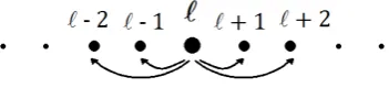
Figure 2.6: Interactions in a 1D next-nearest neighbour model.

Throughout we assume the displacement map u|Z+ belongs to U and identify u(−`) :=

−u(`) for all`_∈Z−. So we can write the atomistic energy in this antisymmetric setting

in the form

Ea +(u) :=

1 2Φ

a 0(u) +

∞

X

`=1

Φa_`(u), (2.4.1)

where theatomistic site energy is

Φa_`(u) := 1 2[φ1(u

0

`) +φ1(u0`+1) +φ2(u0`−1+u0`) +φ2(u0`+1+u0`+2)].

Then we have the identity Ea₍_u_{) = 2}_Ea

+(u). For simplicity we drop the subscript from E+ since we only consider antisymmetric problems. We will use this representation of the atomistic energy because it is the form in which more realistic interatomic potentials are

normally given: see Figure 2.6.

For simplicity we consider only dead load external forces throughout this section.

Letf :Z→Rwithf(`)→0 as |l| → ∞. Then we seek a solution of

ua ∈arg min{Ea₍_u₎_{− h}_{f, u}_i

Z+}. (2.4.2)

Ifua _{is a solution to (2.4.2), it naturally satisfies the Euler–Lagrange equation:}

d dt[E

a₍_u₊_tv₎_{− h}_{f, u}₊_tv_i

Z]

t=0

= 0 for all v∈ U

which is normally written as

hδ_Ea₍_ua₎_{, v}_i₌_h_{f, v}_i

Z+ for all v∈ U. (2.4.3)

2.4.2 Cauchy–Born continuum model

To approximate the atomistic energy, we consider the continuum elasticity model with an energy functional of the form

Ec₍_u_{) =}

Z

R+

W(_|∇u_|)dx,

whereW : (0,∞)→Ris a suitable strain energy function andu∈ U is identified with its

(21)

energy density function

W(F) :=φ1(F) +φ2(2F).

We shall remark that the atomistic and continuum energies are only formally defined, but see [43] for justification. However the first and second variations are well-defined as stated.

And only those are needed for the analysis.

Let us consider a finite element Cauchy–Born model on an infinite atomistic chain. We take the atomistic chain as the set of nodes and consideru:R+→Ras the continuous

piecewise linear interpolation of the discrete displacement mappingu:Z+→R. Then the

Cauchy-Born model is rewritten as

Ec₍_u_{) =} ∞

X

`=1

Φc_`(u), (2.4.4)

where theCauchy–Born site energy is

Φc_`(u) := 1₂W(u0_`) +1₂W(u0_`+1).

For this discretized Cauchy-Born model, we seek

uc∈arg min{Ec₍_u₎_{− h}_{f, u}_i

Z+},

which solves the Euler-Lagrange equation

hδ_Ec(uc), v_i=_hf, v_i_Z₊ for allv_{∈ U},

where

hδ_Ec₍_uc₎_{, v}_i₌ X

`∈Z+

W0(u0_`)v_`0

= X

`∈Z+

{φ0₁(u0_`)v0_`+φ0₂(2u0_`)(2v_`0)_}.

2.4.3 QNL a/c coupling method in 1D

The first method of this kind was formulated by Shimokawa [49]. In this section, for simplicity, we consider the construction valid only for 1D pair interactions, employing an

approximation of bonds rather than site energies. Following [46] we approximate

φ2(u0`+u0`+1)≈

1 2φ2(2u

0 `) +

1 2φ2(2u

0 `+1).

The total energy using QNL coupling is therefore expressed as

Eqnl₍_u_{) :=}_Ea₍_u_{) +} ∞

X

`=K+1

[1 2{φ2(2u

0

(22)

[image:22.595.164.420.88.171.2]

Figure 2.7: Illustration of the constuction of the QNL method, whereA is the atomistic region,_{K, K + 1_} is the interface region and_C is the continuum region

where K is the site where we start approximating atomistic interaction by continuum

models. We can also rewrite_Eqnlas a decomposition into the atomistic region, the interface

region and the continuum region:

Eqnl₍_u_{) =} K−1

X

`=0

Φa_`(u) +

K+1

X

`=K

Φqnl_` (u) +

∞

X

`=K+2

Φc_`(u), (2.4.5)

where Φa_`(u) is defined in (2.4.1), Φc_`(u) is defined in (2.4.4) and

Φqnl_` (u) := 1 2{φ1(u

0

`) +φ2(u0`−1+u0`) +W(u0`+1)},

At the reference state, the first variations of both sides are equal

φ0₂(0)(v0_`+v0_`+1) = 1 2φ

0

2(0)(2v0`) +

1 2φ

0

2(0)(2v`+10 ),

which shows that there are no ghost forces: δ_Eqnl_{(0) = 0 as opposed to other coupling}

methods such as QCE and B-QCE, which is one of the advantages of QNL method. In (2.4.5), the interface atoms_{K, K+ 1_}are called ’quasi-non-local’ because their

interaction with the atomistic region, i.e. the termφ2(u0_K−1+u0_K), is non-local but their

interaction with the continuum region, i.e. the termW(u0_K+1), is local. See Figure 2.7. We approximate the atomistic problem 2.4.2 by

uqnl ∈arg min{Eqnl₍_u₎_{− h}_{f, u}_i

Z+}. (2.4.6)

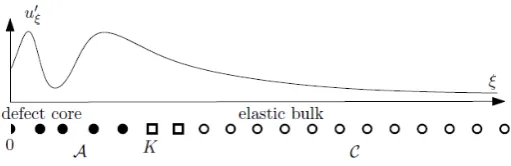
2.4.4 Error Estimation

The general approach for obtaining an error estimate for ua ₋_uqnl _{uses stability and}

consistency results. In the case of modelling crystal defects, we have the following notion

of stability and consistency:

Eh_{, where}_h_{represents a particular approximate model, is}_stable_{on a displacement}

mapu if there exists a constantγ >0 such that

(23)

Aconsistency error estimate η(u) ofEh _at_u_{is often expressed as}

hδ_Eh(u)₋δ_Ea₍_u₎_{, v}_i_._η₍_u₎_k_v_k_,

whereη(u) is determined by discrete derivatives of u. We note thatδ2_E_:_{U → U}∗_{. For example}

hδ2_Ea(u)v, v_i= X

`∈Z+

{φ00₁(u0_`)(v_`0)2+φ00₂(u0_`+u0_`+1)(v_`0 +v_`+10 )2_}.

The stability property comes from the positive-definiteness of the Hessian of the model,

since a solution is a minimizer of the problem_Eh(u)_{− h}f, u_i_Z₊.

With stability and consistency estimates defined above, we can employ the inverse function theorem to obtain the desired error estimates.

Before discussing error estimates, we shall assume that _Ea and _Eqnl satisfy the

following global bounds.

(A) There exist finite constants Ma(j) and M_qnl(j) such that, if Pj_i=1_p1_i = 1, then δj_Ea _and_δj_Eqnl _{satisfy the bounds, for all}_u_{∈ U}_,

hδjEa_u,_v_{i ≤}_M(j) a

j

Y

i=1

kvik`0 pi,

hδjEqnl_u,_v_{i ≤}_M(j) qnl

j

Y

i=1

kvik`0 pi, for all vi ∈ U.

We shall remark that realistically the interatomic potentials are singular as the

distance between any two atoms tends to zero, which contradicts Assumption A. It is purely for the simplicity of analysis. Removing these global bounds does not change the

main concept of the analysis but only adds complications to formulations and proofs.

Recalling the QNL and atomistic energy functionals defined in (2.4.5) and (2.4.1), we can compute the error in the first variation: foru, v_{∈ U},

hδ_Eqnl(u)₋δ_Ea(u), v_i=

∞

X

`∈K+2

2φ0₂(2u0_`)₋φ0₂(u0_`+u0_`+1)₋φ0₂(u_`−10 +u0_`)_}v_`0

+

φ0₂(2u0_K+1)₋φ0₂(u0_K+1+u0_K+2) v_K+10 .

(24)

region. Using Taylor’s expansion we can estimate

|2φ0₂(2u0_`)₋φ0₂(u0_`+u0_`+1)₋φ0₂(u0_`−1+u0_`)_|

≈

φ00₂(2u0_`)

4u0_`₋(u0_`+u_`+10 )₋(u0_`−1+u0_`)_}

+φ0002 (θ)

2

(2(u0_`)−(u0_`+u0_`+1))2+ (2(u0_`)−(u0_`−1+u0_`))2}

=φ00₂(2u0_`)

−u000_`+1 +φ0002(θ)

2

(u00_`+1)2+ (u00_`)2

≤M_qnl|2 _u000

`+1|+M_qnl|3 ₍_u00

`+1)2+ (u00`)2|,

whereu00_` :=u0_`+1−u0_` andu000_` :=u00_` −u00_`−1. Similarly we have

|φ0₂(2u0_K+1)₋φ0₂(u0_K+1+u0_K+2)_{| ≈ |}φ00₂(θ)(2u0_K+1₋u0_K+1₋u0_K+2)_{| ≤}M2 qnl|u

00 K+1|.

Applying the Cauchy-Schwarz inequality gives the consistency estimate,

hδEqnl₍_u₎₋_δ_Ea₍_u₎_{, v}_i

.(ku000k`2_(C)+ku00k2_`4_(C)+|u00K+1|)kv0k`2. (2.4.7)

For stability, we shall first see that the reference state u = 0 is stable in the

atomistic model if and only if it is stable in the Cauchy–Born model. At the reference stateu= 0, a brief calculation shows that

hδ2_Ec₍₀₎_{v, v}_i₌ 1 2W

00₍₀₎

|v0_0|2₊_W00₍₀₎ ∞

X

`=1 |v_`|0 2

=_hδ2_Ea₍₀₎_{v, v}_i₊_φ00 2(0)

∞

X

`=1 |v00_`_|2_,

where we used the fact thatW00(0) =φ00₁(0) + 4φ00₂(0) and the parallelogram identity

|v_`0 +v`+1|0 2_{= 2}_|_v0

`|2_{+ 2}_|_v0

`+1|2_{− |}_v00

`|2. (2.4.8)

For Lennard-Jones type potentials we have thatφ00

2(0)<0, hence

hδ2Ea₍₀₎_{v, v}_{i ≥ h}_δ2_Ec₍₀₎_{v, v}_i_.

It can be checked [13] that

inf

kv0k_`2=1h

δ2_Ec(0)v, v_{i ≥} inf

kv0k_`2=1h

δ2_Ea(0)v, v_i.

Consequently we can state that the reference stateu= 0 is stable in the atomistic model

if and only if it is stable in the Cauchy–Born model.

(25)

(2.4.8) we have

hδ2_Eqnl₍₀₎_{v, v}_i₌_φ00 1(0)

∞

X

`=1

|v0_`|2₊_φ00 2(0)|2v

0 1|2

+φ00₂(0)

K

X

`=1

|v0_`+v_`+1|0 2₊_φ00 2(0)

∞

X

`=K+1 1 2|v

0 `|2₊1

2|v 0 `+2|2

=_hδ2Ec₍₀₎_{v, v}_{i −}_φ00 2(0)

K

X

`=1 |v_`00|2_.

Similar to the Cauchy–Born case, the reference stateu= 0 is stable in the QNL model if

and only if the atomistic and Cauchy–Born Hessians are stable. More generally, we can prove the following result:

Theorem 2.4.1. ([33, Theorem 7.8]) Suppose there exists an atomistic solution ua _to

(2.4.2) that satisfies, for some γa _>₀_,

hδ2_Ea₍_ua₎_{v, v}_{i ≥}_γa_k_v0 k2

`2, ∀v∈ U,

with discrete derivatives decaying as follows, for some α >1/2,

|(ua)(j)(x)_|.x−α+1−j, j= 0,1,2,3.

Then there exists γ₀qnl >0 such that

hδ2Eqnl₍₀₎_{v, v}_{i ≥}_γqnl 0 kv

0 k2

`2, ∀v∈ U.

Then there exists γqnl _>₀ _{such that}

hδ2Eqnl₍_ua₎_{v, v}_{i ≥}_γqnl_k_v0 k2

`2, ∀v∈ U, (2.4.9)

whenK is sufficiently large.

Combining the consistency estimate (2.4.7) and the stability estimate (2.4.9), we

can apply the inverse function theorem (see Theorem 3.4.1) to conclude that there exists a solutionuqnl _{∈ U} _{to (2.4.6) such that}

hδ2_Eqnl(uqnl)v, v_i= 0,

and

k(ua)0₋(uqnl)0_k`2 .k(ua)000k`2_(C)+k(ua)00k2_`4_(C)+|(ua)00K+1|.

2.4.5 Error estimates for other a/c coupling methods

(26)

summa-Recall that the QCE energy is defined in§2.3.4. Suppose β(|x|) = 0 for |x| ≤K

andβ(_|x_|) = 1 for_|x_{| ≥}L, then the consistency error is reduced to be (L₋K)−32 (see [34]

for detailed optimization). The stability is guaranteed up to an error controllable by the

blend width (L−K).

The QCF model introduced in _§2.3.5 is proven not to be stable in the discrete

W−1,2-seminorm in [15]. However, it has been shown that it is stable in the discrete

(27)

Chapter 3 A/C coupling with high-order

finite elements

The theory of high-order finite element methods (FEM) in partial differential equations, and applications in solid mechanics is well established; see [47] and references therein.

However, most work on the rigorous error analysis of a/c coupling has been restricted to

P1 finite element methods; the only exception we are aware of is [45], which focuses on blending-type methods.

In the present chapter we estimate the accuracy of a QNL method employing a P2

FEM in the continuum region against an exact solution obtained from a fully atomistic model. Since stability of QNL type couplings is a subtle issue [41] we will primarily

analyse the consistency errors, taking into account the relative sizes of the fully resolved

atomistic region and of the entire computational domain (Sections 6.1-6.6). We will then optimize these relative sizes as well as the mesh grading in the continuum region in order

to minimize the total consistency error (Section 6.7). We will observe that, using P1-FEM

in the continuum region, the error resulting from FEM approximations is the dominating contributor of the consistency estimates, which implies that increasing the order of the

FEM can indeed improve the accuracy of the simulation. We will show that, using

Pk-FEM withk≥2, the FEM approximation error is dominated by the interface error which comes purely from the coupling construction, and in particular demonstrate that the

P2-FEM is sufficient to achieve the optimal convergence rate for the consistency error. Finally,

assumingthe stability of the G23 coupling (see assumption(A2) in§ 3.2.2, and also [41] why this must be an assumption and cannot be proven), we prove a rigorous error estimate

in§3.5.

Finally, we conduct numerical experiments on a 2D anti-plane model problem to

test our analytical predictions. The numerical results display the predicted error

(28)

[image:28.595.191.406.81.233.2]

Figure 3.1: The lattice and its canonical triangulation.

3.1 Preliminaries

Our setup and notation follows [44]. As our model geometry we consider an infinite 2D

triangular lattice,

Λ :=AZ2, withA= 1 cos(π/3)

0 sin(π/3)

!

.

We define the six nearest-neighbour lattice directions bya1 := (1,0), andaj :=Qj−16 a1, j∈

Z, where Q6 denotes the rotation through the angleπ/3. We supply Λ with anatomistic

triangulation, as shown in Figure 3.1, which will be convenient in both analysis and

nu-merical simulations. We denote this triangulation by_T and its elements byT _{∈ T}. We also denotea:= (aj)6

j=1, andFa:= (Faj)6j=1, forF∈Rm×2.

We identify a discrete displacement map u : Λ _→ Rm, m = 1,2,3, with its

con-tinuous piecewise affine interpolant, with weak derivative∇u, which is also the pointwise derivative on each elementT ∈ T. Form= 1,2,3, the spaces of displacements are defined

as

U0:=

u_|Λ_→Rm: supp(∇u) is compact , and

˙

U1,2:=u_|Λ_→Rm:∇u∈L2 .

We equip ˙U1,2 _{with the}_H1_-seminorm, _k_u_kU₁

,2 :=k∇ukL2₍

R2). From [40] we know that U0

is dense in ˙_U1,2 in the sense that, ifu_∈_U˙1,2_{, then there exist}_u

j ∈ U0such that∇uj → ∇u

strongly inL2_.

Ahomogeneous displacement is a mapuF : Λ→Rm, uF(x) :=Fx, whereF∈Rm×2.

For a mapu: Λ_→Rm, we define the finite difference operator

Dju(x) :=u(x+aj)−u(x), x∈Λ, j∈ {1,2, ...,6}, and

Du(x) := (Dju(x))6j=1.

(3.1.1)

(29)

3.1.1 2D many-body nearest neighbour interactions

We assume that the atomistic interaction is described by a nearest-neighbour many-body

site energy potentialV ∈Cr(Rm×6),r≥5, withV(0) = 0. Furthermore, we assume that

V satisfies the point symmetry

V((−gj+3)6j=1) =V(g) ∀g∈Rm×6.

The energy of a displacementu_{∈ U0}, given by

Ea(u) :=X

`∈Λ

V(Du(`)),

is well-defined since the infinite sum becomes finite. To formulate a variational problem

in the energy space ˙U1,2_{, we need the following lemma to extend}_Ea _{to ˙}_U1,2_.

Lemma 3.1.1. _Ea _{: (}_U0_,_{k∇ · kL}₂₎ _→

R is continuous and has a unique continuous

extension to _U˙1,2, which we still denote by _Ea. Furthermore, the extended _Ea : ( ˙_U1,2,_{k∇ ·} kL2)→_R isr-times continuously Fr´echet differentiable.

Proof. See Lemma 2.1 in [18].

For the sake of analysis we need the following global bounds on the potential V.

Forg∈Rm×6, define the first and second partial derivatives, for i, j= 1, . . . ,6, by

∂jV(g) :=

∂V(g)

∂gj ∈R

m_, _and _∂

i,jV(g) :=

∂2_V₍_g₎ ∂gi∂gj ∈R

m×m_,

and similarly for the third derivatives ∂i,j,kV(g) ∈Rm×m×m. We assume that the second

and third derivatives are bounded

M2 : = 6

X

i,j=1

sup

g∈Rm×6

sup

h1,h2∈R2,

|h1|=|h2|=1

∂i,jV(g)[h1, h2]<∞, and (3.1.2)

M3 : =

6

X

i,j,k=1

sup

g∈Rm×6

sup

h1,h2,h3∈R2,

|h1|=|h2|=|h3|=1

∂i,j,kV(g)[h1, h2, h3]<∞. (3.1.3)

With the above bounds it is easy to show that

6

X

i=1

|∂iV(g)−∂iV(h)| ≤M2 max

j=1,...,6|gj−hj|,

6

X

i,j=1

|∂i∂jV(g)−∂i∂jV(h)| ≤M3 max

k=1,...,6|gk−hk|, forg,h∈R

(30)

3.1.2 The variational problem

We add an external potentialf _∈Cr( ˙_U1,2) with ∂_u(`)f(u) = 0 for all _|`_{| ≥}Rf, where Rf

is some given radius, and f(u+c) =f(u) for all constants c. For example, we can think off modelling a substitutional impurity. See also [30, 39] for similar approaches.

We then seek the solution to

ua _∈_{arg min}

Ea₍_u₎₋_f₍_u₎_|_u_∈_U_˙1,2 _. _(3.1.5)

Foru, ϕ, ψ_∈_U˙1,2 we define the first and second variations of _Ea by

hδ_Ea(u), ϕ_i:= lim

t→0t −1₍

Ea(u+tϕ)_{− E}a(u)),

hδ2_Ea(u)ϕ, ψ_i:= lim

t→0t −1₍

hδ_Ea(u+tϕ), ψ_{i − h}δ_Ea(u), ψ_i).

We use analogous definitions for all energy functionals introduced in later sections.

3.1.3 The Cauchy–Born Approximation

The Cauchy–Born strain energy function, corresponding to the interatomic potentialV is

W(F) := 1 Ω0

V(Fa), forF∈Rm×2,

where Ω0 := √

3/2 is the volume of a unit cell of the lattice Λ. Thus W(F) is the energy per volume of the homogeneous latticeFΛ.

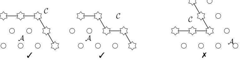
3.1.4 The G23 coupling method

Let_{A ⊂}Λ denote the set of all lattice sites for which we want to maintain full atomistic

accuracy. We denote the set of interface lattice sites by

I :=

`_∈Λ_{\ A}`+a_j ∈ Afor somej ∈ {1, . . . ,6}

and we denote the remaining lattice sites by C := Λ\(A ∪ I). Let Ω` be the Voronoi

cell associated with site `. We define the atomistic, interface and continuum regions

respectively by

Ωa := [

`∈A

Ω`, Ωi:=

[

`∈I

Ω`, and Ωc:=R2\

[

`∈A∪I

Ω`;

see Figure 3.2 for a visualisation.

A general form for the GRAC-type a/c coupling energy [16, 44] is

Eac₍_u_{) =}X

`∈A

V(Du(`)) +X

`∈I

V (_R`Dju(`))6j=1

+

Z

Ωc

(31)

[image:31.595.163.435.82.213.2]

∂Ωc : Atomistic node (A) : Interface node (I) : Continuum node (_C)

Figure 3.2: The domain decomposition with a layer of interface atoms.

A

3 C

A

3 C

A

C

7

Figure 3.3: The first two configurations are allowed. The third configuration is not allowed as the interface atom at the corner has no nearest neighbour in the continuum region, and should instead be taken as an atomistic site.

where _R`Dju(`) := P6_i=1C`,j,iDiu(`). For the sake of brevity of notation we will often

write

V_`i(Du(`)) :=V (R`Dju(`))6j=1

.

The parametersC`,j,iare to be determined in order for the coupling scheme to satisfy the

“patch tests”:

Eac _is_{locally energy consistent} _{if, for all}_F_∈

Rm×2,

V_`i(Fa) =V(Fa) _∀`_{∈ I}. (3.1.6)

Eac _is_{force consistent} _{if, for all}_F_∈

Rm×2,

δ_Eac₍_u

F) = 0, (3.1.7)

whereuF ∈U˙1,2 anduF(x) :=Fxfor all x∈R2.

Eac _is_{patch test consistent} _{if it satisfies both (3.1.6) and (3.1.7).}

Following [44] we make the following standing assumption (see Figure 3.3 for

ex-amples).

(A0)Each vertex`∈ I has exactly two neighbours in_I, and at least one neighbour in _C.

[image:31.595.107.492.254.351.2]

(32)

2 3 2

3 2 3 2

3

2 3

1

[image:32.595.182.416.83.232.2]

1

Figure 3.4: The geometry reconstruction coefficentsλx,j at the interface sites.

by

R`Dju(`) := (1−λ`,j)Dj−1u(`) +λ`,jDju(`) + (1−λ`,j)Dj+1u(`),

λx,j :=

(

2/3, x+aj ∈ C

1, otherwise ;

(3.1.8)

see Figure 3.4. The resulting coupling method is called G23 and the corresponding energy

functional_Eg23:

Eg23₍_u_{) :=}X

`∈A

V(Du(`)) +X

`∈I

V (R`Dju(`))6j=1

+

Z

Ωc

W(∇u(x)) dx, (3.1.9)

where R`Dju(`) is defined as (3.1.8). This choice of coefficients (and only this choice)

leads to patch test consistency (3.1.6) and (3.1.7). We refer to [44] for a detailed proof.

For future reference we decompose the canonical triangulation_T as follows:

TA: ={T ∈ T |T∩(I ∪ C) =∅}, TC: ={T ∈ T |T∩(I ∪ A) =∅} and TI : =T \(TC∪ TA).

(3.1.10)

3.1.5 Notation for a P2 finite element scheme

In the atomistic and interface regions, the interactions are represented by discrete dis-placement maps, which are identified with their linear interpolant. Here, we identify the

displacement map with its P1 interpolant. No approximation error is committed.

On the other hand, in the continuum region where the interactions are approxi-mated by the Cauchy–Born energy, we could increase the accuracy by using Pp-FEM with

p >1. In later sections we will review that the Cauchy–Born approximation yields a 2nd-order error, whereas employing the P1-FEM in the continuum region would reduce the accuracy to first order. In fact, we will show that, with optimized mesh grading, P2-FEM

is sufficient to obtain a convergence rate that cannot be improved by other choices of

(33)

costs but yield the same error convergence rate (see§3.2.5). LetK >0 denote the inner radius of the atomistic region,

K := supr >0_{| Br}_∩Λ_{⊂ A} ,

where_Br denotes the ball of radius r centred at 0. In order for the defect to be contained

in the atomistic region we assume throughout thatK_≥Rf.

Let Ωh denote the entire bounded computational domain and N > 0 denote the

inner radius of Ωh, i.e.,

N := sup

r >0_{| Br}_⊂Ωh .

LetTh be a finite element triangulation of Ωh which satisfies that, forT ∈ Th,T is closed

and

T_∩(_{A ∪ I})₆=_∅ _⇒ T _{∈ T}.

In other words, _Th and _T coincide in the atomistic and interface regions, whereas in the

continuum region the mesh size may increase towards the domain boundary. Define the

mesh size h(x) := diam(T) with x ∈ T. The optimal rate at which the mesh size h

increases will be determined in later sections.

We note that the concrete construction of _Th will be based on the choice of the

domain parameters K and N; hence, when emphasizing this dependence, we will write

Th(K, N). We assume throughout that the family (_Th(K, N))K,N is uniformly shape-regular, i.e., there exists c >0 such that,

diam(T)2_≤c|T|, ∀T ∈ Th(K, N),∀K≤N. (3.1.11)

This assumption eliminates the possibility of extreme angles on elements, which would

deteriorate the constants in finite element interpolation error estimates. For the most part we will again drop the parameters from the notation by writing _Th _{≡ Th}(K, N) but

implicitly will always keep the dependence.

Similar to (3.1.10), we define the atomistic, interface and continuum elements as

Ta

h,Thi and Thc, respectively. Note thatTha=TA and Thi =TI. We also let Nh denote the

number of degrees of freedom of_Th.

We define the finite element space of admissible displacements as

Uh:=

u∈C(R2;Rm)|supp(u)⊂Ωh, u|T ∈P1(T) for T ⊂ Tha∪ Thi and

u|T ∈P2(T) for T ⊂ Thc .

(3.1.12)

In definingUh we have made two approximations to the class of admissible displacements: (1) truncation to a finite computational domain and (2) finite element coarse-graining.

The computational scheme is to find

ug23_h ∈arg minEg23₍_u

(34)

Remark 3.1.2. Uh is embedded inU0 via point evaluation. Through this identification,

f(uh) is well-defined for all uh ∈ Uh.

We will make this identificationonlywhen we evaluatef(uh). The reason for this

is a conflict when interpreting elements uh as lattice functions due to the fact that we

identify lattice functions with their continuous interpolants with respect to the canonical

triangulation _T, which would be different from the function uh itself. However, for the

evaluation off(uh) this issue does not arise.

3.2 Summary of results

3.2.1 Regularity of ua

The approximation error analysis in later sections requires estimates on the decay of the elastic fields away from the defect core. These results follow from a natural stability

assumption:

(A1) The atomistic solution is strongly stable, that is, there exists C0 >0 such that

hδ2_Ea(ua)ϕ, ϕ_{i ≥}C0_k∇ϕ_k2_L2, ∀ϕ∈U˙1,2, (3.2.1)

whereua _{is a solution to (3.1.5).}

Corollary 3.2.1. Suppose that (A1) is satisfied, then there exists a constant C > 0

such that, for1≤j ≤r−2,

|Djua₍_`₎_{| ≤}_C_|_`_|−1−j_.

Proof. See Theorem 2.3 in [18].

3.2.2 Stability

In [41] it is shown that there is a “universal” instability in 2D interfaces for QNL-type a/c

couplings: it is impossible to prove in full generality thatδ2_Eg23₍_ua_{) is a positive definite}

operator, even if we assume (3.2.1). Indeed, this potential instability is universal to a wide class of generalized geometric reconstruction methods. However, it is rarely observed in

practice. To circumvent this difficulty, we make the following standing assumption:

(A2) The homogeneous lattice is strongly stable under the G23 approximation, that is, there existsC₀g23>0 which is independent ofK such that, forKsufficiently large,

hδ2Eg23₍₀₎_ϕ

h, ϕhi ≥C0g23k∇ϕhk 2

L2, ∀ϕh∈ Uh. (3.2.2)

Since (3.2.2) does not depend on the solution it can be tested numerically. But a

precise understanding under which conditions (3.2.2) is satisfied is still missing. In [41] a

(35)

replace this assumption, however we are not yet able to extend this stabilizing method for interfaces with corners, such as the configurations discussed in this thesis.

3.2.3 Main results

To state the main results it is convenient to employ a smooth interpolant to measure the regularity of lattice functions. In Lemma 3.5.1, we define such an interpolant ˜u∈C2,1(R2)

for u _{∈ U0}, for which there exists a universal constant ˜C such that, for all q _∈ [1,_∞],

0≤j≤3,

|Dju(`)_{| ≤}C˜_k∇ju˜_kL1_(ω

`) and k∇

j_u_˜_kL

q_(T₎≤C˜kDjuk`q_(Λ∩T₎

whereω` :=`+A(−1,1)2.

3.2.3.1 Consistency error estimate

In (3.4.6) we define a quasi-best approximation operator Πh :U0 → Uh, which truncates

an atomistic displacement to enforce the homogeneous Dirichlet boundary condition, and

then interpolates it onto the finite element mesh.

Our main result is the following consistency error estimate.

Theorem 3.2.2. If ua _{is a solution to} _(3.1.5) _{then we have, for all} _ϕ

h∈ Uh,

hδEg23_(Π

hua), ϕhi.

k∇2_u_˜a_kL

2_(Ωi₎+k∇3u˜akL2_(Ωc₎+k∇2u˜ak2_L4_(Ωc₎

+_kh2_∇3_u_˜a_kL

2_(Ωc

h)+k∇u˜

a_kL

2₍

R2\BN/2)

+N−1_kh2_∇2_u_˜a_kL

2_(B

N\BN/2)

k∇ϕ_hkL2₍

R2\Ωa),

(3.2.3)

where Ωc_h corresponds to the continuum region of Ωh, and h(x) := diam(T) with x∈T ∈ Th.

3.2.3.2 Optimizing the approximation parameters

Before we estimate the error_k∇u˜a_−∇_ug23

h kL2, we optimize the approximation parameters

in the computational scheme. This means that the radiusK of the atomistic region, the radiusN of the entire computational domain and the mesh size h should satisfy certain

balancing relations. We only outline the result of this optimisation and refer to_§3.5.7 for

the details.

Due to the decay estimates on ˜ua _{(cf. Corollary 3.2.1) the dominating terms in}

(3.2.3) turn out to be

k∇2_u_˜a_kL

2_(Ωi₎ .K−5/2 and k∇u˜akL2₍

R2\BN/2).N

−1

(36)

β N Nh consistency error P2-FEM 1,3

2

K5/2 K2 _K−5/2

P1-FEM 1,3 2

[image:36.595.171.422.83.133.2]

K2 _K2 _K−2

Table 3.1: Quasi-optimal relations between approximation parameters for P2-GR23 and, for comparision, for P1-GR23.

(We will see momentarily that the mesh size plays a minor role.) These two terms result

from the nature of the coupling scheme and the far-field truncation error. In particular, both of these cannot be improved by the choice of discretisation of the Cauchy–Born

model, e.g., order of the FEM. We also note that, if we had employed a P1-FEM, the only

different terms in the analog of (3.2.3) arekh∇2_u_˜a_kL₂

(Ωc₎rather thankh2∇3u˜akL2_(Ωc₎, and

N−1_k_h_∇_u_˜a_kL

2_(B

N\BN/2) rather than N

−1_k_h2_∇2_u_˜a_kL

2_(B

N\BN/2), hence the limiting factor

would have been_kh_∇2_u_˜a_kL

2_(Ωc₎.K−4 (at best); cf. §3.5.7.

We can balance the two terms in (3.2.4) by choosingN ≈K5/2. It then remains to determine a mesh-size so that the finite element error contribution,

kh2_∇3u˜a_kL2_(Ωc

h) and N

−1

kh2_∇2u˜a_kL2_(B

N\BN/2)

remains small in comparison. We show that the scalingh(x)_≈|x|_Kβ is a suitable choice, with 1< β <3/2, under which both terms become of order O(K−3).

Thus, we have determined the approximation parameters (K, N, h) in terms of a

single parameterK. The quasi-optimal relations for P2-FEM discretization of the Cauchy–

Born model are summarised in Table 3.1.

Corollary 3.2.3. Suppose that N, h satisfy the relations of Table 3.1, the consistency error estimate (3.2.3) in terms of the number of degrees of freedom _Nh can be written as

kδEg23_(Π

hua)kU−1,2 .N_h−5/4. (3.2.5)

3.2.3.3 Error estimate

To complete our summary of results, we now use the Inverse Function Theorem to obtain

error estimates for the strains and the energy.

(37)

the error estimates

k∇ua_{− ∇}_ug23

h kL2 .N −5/4

h , and (3.2.6)

[Ea(ua)−f(ua)]−[Eg23(u

g23

h )−f(ug23)]

.N

−7/4

h , (3.2.7)

where Nh is the number of degrees of freedom and scales as Nh∼K2_.

Remark 3.2.5. The analogous estimates of P1-GR23 to (3.2.6) and (3.2.7) are _N_h−1

andNh−2 respectively.

3.2.4 Setup of the numerical tests

For our numerical tests, we consider an anti-plane displacementu: Λ→R. We choose a

hexagonal atomistic region Ωa with side length K and one layer of atomistic sites outside

Ωa as the interface. To construct the finite element mesh, we add hexagonal layers of elements such that, for each layerj,h(layer j) = (_|x|/K)β, with β = 1.4; see Figure 3.5.

The procedure is terminated once the radius of the domain exceeds N = _dK5/2_e_{. This}

construction guarantees the quasi-optimal approximation parameter balance to optimise the P2-FEM error. The derivation is given in Section 3.5.7.

In our tests we compare the P2-G23 method against

(1) a pure atomistic model with clamped boundary condition: the construction of the

domain is as in the P2-G23 method, but without continuum region;

(2) a P1-G23 method: the construction is again identical to that of the P2-G23 method,

but the P2-FEM in the definition of _Uh is replaced by a P1-FEM. The same mesh

scaling as for P2 is used (see also [16] where this is shown to be quasi-optimal).

The site potential is given by a nearest-neighbour embedded atom toy model,

V(Du) :=G 6

X

i=1

ρ(|Diu(`)|)

!

with G(s) :=s+1₂s2 _and _ρ₍_r_{) := sin}2₍_rπ_{). This is a simplified anti-plane toy model as}

used in [18], which absorbs the pair interaction into the embedding term.

The external potential is defined by hf, ui = 10(u(0,0)−u(1,0)), which can be thought of as an elastic dipole. A standard steepest descent method, preconditioned with

a finite element Laplacian (see, for example [3]) and fixed (manually tuned) step-size, is

used to find a minimizer ug23_h of Eg23₍_u₎₋_f₍_u_{) (see (3.1.9) for the formulation of} _Eg23₎

usinguh= 0 as the starting guess.

In order to compare the errors, we use a comparison solution with atomistic region

size 3K and other computational parameters scaled as above.

(38)

-15 -10 -5 0 5 10 15 -10

[image:38.595.191.404.79.278.2]

-5 0 5 10

Figure 3.5: An example of the computatioanl mesh. The the vertices marked by ”_•” are the atomistic sites; the vertices marked by ”_∗” are the interface sites.

(1) the numerical tests confirm the analytical predictions for the geometry and the

energy-norm errors, but the experimental rates for the energy error are better than

the analytical rates. Similar observations were also made in [18].

(2) With our specific setup, the improvement of the P2-GR23 over P1-GR23 is clearly observed when plotting the error against #_{A ∝ Nh}, but when plotted against _Nh

the improvement is only seen in the asymptotic regime. This indicates that further

work is required, such as a posteriori adaption, to optimise the P2-GR23 in the pre-asymptotic regime as well.

3.2.5 Extension to high-order FEM

If we apply higher-order FEM in the continuum region, then to extend our error analysis

we would need a smooth interpolant ofu_{∈ U0} with higher regularity than ˜u_∈C2,1(R2).

A suitable extension given in [30] is, for arbitraryn, aCn,1 piecewise polynomial of degree 2n+1 with properties analogous to those stated in Lemma 3.5.1. The resulting higher-order

decay rate _|∇ju˜a₍_x₎_| _._|_x_|−j−1 _{(cf. Corollary 3.2.1) indicates that the use of high-order}

FEM could be beneficial.

However, as we have pointed out in_§ 3.5.7, if we employ the mesh gradingh(x) =

(_|x_|/K)β with 1< β <3/2 in the continuum region, the total approximation error cannot

be improved by using Pp-FEM withp >2, since the dominating term is the interface error

k∇2_u_˜a_kL

2_(Ωi₎ for p ≥ 2, which results from the construction of G23 coupling and is not

affected by the choice of FEM.

If we consider a coarser mesh for high-order FEM in hopes of reducing the number of degrees of freedom, i.e., choosingβ_≥3/2, then applying analogous calculations to those

(39)

100 101 102 10-5

10-4 10-3 10-2

10-1 Point Defect : Geometry Error

[image:39.595.134.454.92.361.2]

ATM G23-P2 G23-P1

Figure 3.6: Error in energy norm plotted against #A. We clearly observe the predicted rate of convergence.

101 102 103 104 105

10-5 10-4 10-3 10-2

10-1

Point Defect : Geometry Error

ATM

G23-P2

G23-P1

[image:39.595.121.472.424.719.2]

(40)

100 101 102 10-8

10-7 10-6 10-5 10-4 10-3 10-2

10-1 Point Defect : Energy Error

[image:40.595.137.455.104.368.2]

ATM G23-P2 G23-P1

Figure 3.8: The energy error plotted against #_A. The observed rate of convergence is better than the rate predicted in Theorem 3.2.4.

Nh

101 102 103 104 105

j

E

h(

7

uh

)

!

E

a(

7

u

a)j

10-8 10-7 10-6 10-5 10-4 10-3 10-2

10-1 Point Defect : Energy Error

ATM G23-P2 G23-P1

9Nh!1

9N!2 h

9N!52 h

[image:40.595.131.462.437.709.2]

Atomistic to continuum coupling

warwick.ac.uk/lib-publications

A Thesis Submitted for the Degree of PhD at the University of Warwick

Permanent WRAP URL:

http://wrap.warwick.ac.uk/101783

Copyright and reuse:

This thesis is made available online and is protected by original copyright.

Please scroll down to view the document itself.

Please refer to the repository record for this item for information to help you to cite it.

Our policy information is available from the repository home page.

M A

O

D

C

S

Atomistic-to-continuum coupling

Huan Wu

Thesis

Doctor of Philosophy

Mathematics Institute

The University of Warwick

Contents

Acknowledgments

Declarations

Abstract

Chapter 1

Introduction

Chapter 2

Background

2.1

Interatomic potentials

2.2

Crystals and defects

2.3

Atomistic-to-continuum models

ghost forces

A

C

2.4

General framework for analyzing A/C coupling models:

an example in 1D

Chapter 3

A/C coupling with high-order

finite elements

3.1

Preliminaries

A

3

C

A

3

C

A

C

7

1

1

1

1

1

1

1

1

1

1

3.2

Summary of results

Point Defect : Geometry Error