Small Sample Estimation in Dynamic Panel Data Models: A Simulation Study

doi:10.4236/ojs.2011.12007 Published Online July 2011 (http://www.SciRP.org/journal/ojs)

Small Sample Estimation in Dynamic Panel Data Models:

A Simulation Study

Lorelied. A. Santos, Erniel B. Barrios

School of Statistics, University of the Philippines Diliman, Quezon City, Philippines E-mail: lorelie.santos@gmail.com, ernielb@yahoo.com

Received March 17, 2011; revised April 2, 2011; accepted April 10, 2011

Abstract

We used simulated data to investigate both the small and large sample properties of the within-groups (WG) estimator and the first difference generalized method of moments (FD-GMM) estimator of a dynamic panel data (DPD) model. The magnitude of WG and FD-GMM estimates are almost the same for square panels. WG estimator performs best for long panels such as those with time dimension as large as 50. The advantage of FD-GMM estimator however, is observed on panels that are long and wide, say with time dimension at least 25 and cross-section dimension size of at least 30. For small-sized panels, the two methods failed since their optimality was established in the context of asymptotic theory. We developed parametric bootstrap ver-sions of WG and FD-GMM estimators. Simulation study indicates the advantages of the bootstrap methods under small sample cases on the assumption that variances of the individual effects and the disturbances are of similar magnitude. The boostrapped WG and FD-GMM estimators are optimal for small samples.

Keywords:Dynamic Panel Data Model, Within-Groups Estimator, First-Difference Generalized Method of

Moments Estimator, Parametric Bootstrap

1. Introduction

Panel data combine cross-sectional and time series in-formation. Since the temporal dependencies for each unit could vary significantly, a dynamic parameter is desir-able to relax the parametric constraints into the model. Dynamic panel data (DPD) model postulates the lagged dependent variable as an explanatory variable. Just like in univariate time series analysis, modeling the depend-ency of the time series on its past value(s) gives valuable insights on the temporal behavior of the series. [1] noted that many economic relationships are dynamic in nature and the panel data allow the researcher to better under-stand the dynamics of structural adjustment exhibited by the data.

A good number of dynamic panel data estimators have been proposed and thoroughly characterized in the lit-erature. The within-group (WG) estimator, among the early estimation method for DPD, provides consistent estimate for static models. In DPD models, [2] showed that the WG estimator of the coefficient of the lagged dependent variable parameter is downward biased and the bias only disappears as the number of time units grows larger. Thus, the WG estimator is known to be

biased whenever the time-dimension is fixed, even if the cross-section dimension is large.

T N

The inconsistency of the WG estimator leads to the development of DPD coefficient parameter estimators that are consistent for large and fixed or large , e.g., the use of instrumental variables (IV). For the IV estimators, [3] used either the dependent variable lagged two periods or its first-differences as instruments. Even the development of the generalized method of moments (GMM) estimators for DPD coefficient parameters is based on the IV approach. [4] proposed GMM estimator that uses all available lags at each period as instruments for the equations in first differences, this is now known as the first-difference generalized method of moments estimator (FD-GMM). [5] proposed the level GMM es-timator which is based on the level of the model and uses lagged difference variables as instruments. [6] further proposed the now called system GMM estimator which uses both the lags of the level and first difference as in-struments.

N T

numer-L. A. SANTOS ET AL. 59

T ous studies on the properties of dynamic panel data model but are mostly focusing on data sets with large cross-section and small time dimensions. Other studies highlight datasets with sizeable cross-section dimensions and moderately-sized time dimensions.

We used intensive simulations to investigate both the small and large sample properties of two of the simplest and oldest DPD estimators, the within-groups and first-difference generalized method of moments estima-tors of the AR(1) DPD model. We also propose the use of parametric bootstrap procedure in the WG and FD-GMM for the boundary scenario, i.e., when asymp-totic optimality of WG and FD-GMM fail.

As [11] pointed out, the application of bootstrap meth- odology in panel data analysis is currently in its embry- onic stage. The bootstrap estimators proposed in this study can answer the possible limitations of the estima- tors by [8]. Over a short period, it is common for proc- esses over time to be easily affected by random shocks. Thus, if long period data are used, it is very likely that structural change will manifest and the modeler will ei-ther incorporate the change into the model (more com-plicated), or analyze the series by shorter periods, lead-ing to small sample data where the proposed estimator is applicable.

2. Dynamic Panel Data Model

Suppose the dynamic behavior of a time series for unit i (yit) is characterized by the presence of a lagged

depend-ent variable among the regressors, i.e.

, 1 1, , 1, ,

it i t it it

y y  x i  N t  (1) where  is a constant, xit is vector of

ex-planatory/exogenous variables, and 1K

 is K1 vector of regression coefficients. _it follows a two-way error component model _it   _{i t}_it where _i and _t

are the (unobserved) individual and time specific effects,

which are assumed to stay constant for given over and for a given over , respectively; and _it

i t

t i 

repre-sents the unobserved random shocks over i and t. The unobserved individual-specific and/or time-specific ef-fects i and t, are assumed to follow either the fixed

effects model (FE) or the random effects model (RE). If Equation (1) assumes a RE model and if it follow

one-way error component model it i it

a

   individual and time specific effects are

 , then the



2



~ IID 0,

i 

 

and



2



it v each other and

among themselves. When i

~

v IID 0, in pendde ent of

 and t are eated

fixed constants, the usual assumptions are

tr as





_2

 

1 i

i and

1N



N O 1

 

1 T 2



1



t

T



_t1 . [12], [1] and [13] give detailed discussions on dynamic panel data models.

O 

Consider the following AR(1) dynamic panel data model without exogenous variable

1 1, 2, , ; 1, 2, ,

it it i it

y y    i  N t  T (2) where yit is the dependent variable,  is the

regres-sion coefficient (parameter of interest) with  1, i

is the unobserved heterogeneity or individual effect which has mean 0 and variance _2



0



and _{it is} unobserved disturbance with mean 0 and variance

 

0 2

_  . To facilitate the computations of estimators of model 2, let xit yit1;yi 



yi1, , yiT



’;



1 iT



i  xi , ,x

x  ’; v_i 



_i1, ,_iT



’; and _T 



1,,1



’ (a

 1

T vector of ones). Equation (2) can be written as

i i i T  i

y x v (3)

[8] considered several estimators of  , e.g., the within group/covariance (WG) estimator (also called fixed effects (FE) estimator), covariance (CV) estimator (or least squares dummy variable (LSDV) estimator), and the first-difference generalized method of moments (FD-GMM) estimator (one-step level GMM estimator proposed by [4]). In the computation of ˆWG and

FD-GMM ˆ

 further notations are used:





































1 2

1 1 1 1 1

1

1 1 1 1 1

1 1 1 1

0 1

2 2 2

1 1

diag , ,

2

1 1

0 0 0 1

2 2

0 0 0 0 1 1

T T T T T

T T T T

T T

 _{    } 

 _{    } 

 

 

   

 _{   } 



  _{ }

 _{ }  _{ }

  _{ }

 _{ } 

 

 



 

 



 

     





A 2











 



*

1 1

... 1

it it it iT

T t

x x x

T t T t  x

 



     

1 2 1 i i i iT       _{ }     z z Z z



1,...,



1, 2 1 2

it xi xit t x xt t xNt t z zt t Nt

   

       

 _  _{  }

z x Z z 

[8] defined the WG estimator as

1 WG

1 ˆ

N i T i i

N i T i i      





x Q y

x Q x (4) where QT IT t lT T T , T is called the WG

opera-tor of order T. WG estimator may also be written in terms of the forward orthogonal deviations operator

Q

A, an upper triangular-like matrix, with dimension

and with the following characteristics:

, T1 and . Let and

, then WG estimator is given by



T 1



T  

A A Q

 _

y Ay

T

x

 

AA I Al_T 0 xA

WG ˆ

  x y _{ }

x x (5) [8] further analyzed an asymptotically efficient FD-GMM estimator given by









1 FD-GMM 1 ˆ              

x Z Z Z Z y

x Z Z Z Z x

(6)

where . A computationally useful al-ternative expression for



1

, , N 

 

 

Z Z Z

ˆ



FD GMM  _ is:

1 1 FD-GMM 1 1 ˆ T

t t t t

T

t t t t            





x M y x M x

(7)

where _t and _t are the vectors whose ith elements are and it, respectively,

t t t t and t is the matrix

whose ith _{row is . As pointed by [8], is} non-singular when , but the projections involved remain well defined in any case. Without loss of general-ity, the condition 1 was maintained because the FD-GMM estimator is motivated in a situation where T is smaller than N and it is straightforward to extend the results in their paper to allow for any combination of values of T and N by considering a generalized formula-tion of 7 using t t t t , where t t



x y

1 Z

it

Z N T



1 N





Z Z it  x



_



 Z  y  1 

N T

M Z

t 

M Z Z Z





Z

N t  Z Z



t









t IN

N

Z Z is the Moore-Penrose inverse of



_{t t} . In this way,

t t t t t if t and if .

Thus, the contribution of terms with to the FD- GMM formula coincide with the corresponding terms for WG.  Z Z N





M Z ZZ



1Z  M

t tN

[8] derived the asymptotic properties of several

dy-namic panel data estimators namely, within groups (WG), first-difference generalized method of moments (FD-GMM), limited information maximum likelihood (LIML), crude GMM and random effects ML estimators of the AR(1) parameter of a simple DPD model with random effects.

As observed by [8], ˆ_WG is consistent for , regardless of . However, as , the asymptotic distribution of WG

T   N

ˆ N 

 may contain an asymptotic bias term, depending on the relative rates of increase of

and . When

T N 0 l im



T N



 



, the asymptotic variance of WG estimator is the same as the of GMM estimator and they have similar (negative) asymptotic biases in which for WG has order 1



T . On the other hand, ˆ_FD-GMM is a consistent estimator for  as both N and T , provided that





2   

logT N0. Also, the number of the FD-GMM orthogonality conditions q T



1 2



FD-G

ˆ T

  tends to infin-ity as T  . The F  MM is asymptotically nor-mal, provided that T   and lim



T N



0. When





0 lim T N   , the asymptotic variance of FD- GMM estimator is the same as the WG estimator and they have similar expression for their (negative) asymp-totic biases in which for FD-GMM has order



1



N. When TN, the asymptotic bias of GMM is smaller than the bias of WG. When , the two asymptotic biases are equal and when

T N 0



N T , the asymptotic bias in the WG estimator disappears.

From a simulation study, [7] observed that the vari-ance of the WG estimators is usually much smaller than the variance of consistent GMM estimators, see [2], [7-9], [14], and [8] for further details.

3. The Bootstrap Method

The bootstrap is a useful tool for estimation in finite samples. Bootstrap procedure entails the estimation of parameters in a model through resampling with a large number of replications, [15]. [16] developed the idea of bootstrap procedure known as a nonparametric method of resampling with replacement and it stems from older resampling methods such as the jackknife method and delta method. Originally, the bootstrap requires inde-pendent observations, i.e., consisting of observa-tions 1

x n

x , x2, …, xn, a random sample from the true

distribution F x

 

generating the data. The data gener-ates the empirical distributionF x

 

, a discrete distribu-tion that assigns equal probability to the observations of the observed sample, hence,

n

 

1

 

2

 

. The bth bootstrap

sample is a vector

1 n

p x p x  n

b p x

 

  



x consisting of observations ,1

b

n

x , x_b,2, …, x_{b n,} (b1, , B), obtained by sampling with replacement B times from the empirical distribution

 

estima-L. A. SANTOS ET AL. 61

tor of a parameter in a particular model is computed, resulting to t x

 

₁ ,

 

, …,

2

t x

 

B

t x _{, where t}

 

x is an estimator of a parameter, say θ.

For time series models, the sieve bootstrap and the block bootstrap are recently introduced. The sieve boot-strap starts by fitting the most adequate model and the behavior of the empirical distribution of the residuals is analyzed. The bootstrap errors _t _{are generated by}

re-sampling T k times from the empirical distribution

 

t

F  , . In order to generate the bth _bootstrap sample b  1,b 1,b T b, , each element of

k p y y

_  _,  _{, , y} _

y b



y is determined by the recursion , i 0 i t i b, t b,

p

yt b y 

, ,y_{T b}

1 2 1 c c cN cN      1, , _b, y y

 







 , where the starting values for t b, are set to zero and the first generated values are thrown away, so that the

needed bth _{bootstrap sample is}

obtained.



1, b b _  , 1 , 1 1, 1 , 1 N T N T y y y y      y y k

On the other hand, the block bootstrap resamples from overlapping blocks of consecutive observations to gener-ate the bootstrap replicgener-ates, see [17] and [15] for a more comprehensive discussion of bootstrap methods for time series models.

To define the bootstrap for dynamic panel data models, suppose is defined as measurements from different cross-section units of the population over different time periods, so that the data can be represented by

y

11 1 1,

21 2 2,

1,

, ,

T T

T T

PD

N N T

N N T

t y y y y  12 22 1,1 ,1 1 2 N N t tT y y y y y y y y

 1,2

2 1 tT                             _ _  y y y y          y     y y y   y  N (8) The bth _{bootstrap sample is the T matrix}

b  y , T b T b , given by

1 1, ,

2 2, ,

1, , , b b b 1, 1, 1,1, ,1, 1, 2, 1, , 12, 22, 1,2, ,2, b b b b 1, 1, 2, 1, 1, 1, , 1, T T

N b N

N b c b c b b b y y y y y y y y                      b N b t          

y1,b t1,

N T

N T b

y y y y          1,

tT b

y y b N N T cN cN y                  y y y y y ,

b tT b

  y

T b b y y y                    N T (9)

b is generated by doing the AR-sieve bootstrap pro-cedure for panel data. [11] identified five bootstrap methodologies for panel data namely: i.i.d. bootstrap,

individual bootstrap, temporal bootstrap, block bootstrap and double resampling bootstrap. The i.i.d bootstrap re-fers to the bootstrap procedure defined by [16]. Each of the



y

 elements of the observed data matrix yPD is

given 1 NT probability in the empirical distribution

 

F y . The elements of the bth _{bootstrap sample} b



y in (9) are obtained by resampling with replacement from the empirical distribution F y

 

.

The rows of y_PD in (8) are resampled with replace-ment in order to determine the bth _{bootstrap sample}

b



y of the form in (9) in the individual bootstrap procedure. On the other hand, in the temporal bootstrap procedure, the columns of yPD in (8) are resampled with

replace-ment in order to create the bth _{bootstrap sample} b



y of the form (9). The resampling procedure for the block bootstrap is in the temporal dimension, so that the data matrix of the form (8) is used. The difference between the block bootstrap and the temporal bootstrap is on the sampling of blocks of columns of yPD in (8) instead of

single column/period in the temporal bootstrap case. Let T Kl, where is the length of a block and thus, there are

l

K non-overlapping blocks. Block bootstrap resam-pling entails the construction of _b such as (9) with columns obtained by resampling with replacement the

non-overlapping blocks columns of



y

K yPD in (8).

Given the data matrix y_PD, double resampling is a procedure that constructs the bth _{bootstrap sample}

b



y by resampling columns and rows of yPD. Two schemes

can be chosen, the first is a combination of individual and temporal bootstrap and the second is a combination of individual and block bootstrap. Therefore, as the name of this bootstrap procedure implies, it involves two/dou- ble stages. The first stage is to construct an intermediate bootstrap sample b



y by performing individual boot- strap. The second stage uses the intermediate bootstrap sample _b

y as a matrix where either temporal bootstrap or block bootstrap is applied to produce the bth _bootstrap sample yb.

4. Bootstrap Procedure for Dynamic Panel

Data Estimators

While the literature clearly illustrates the asymptotic op-timality of WG and FD-GMM estimators, there are doubts on their performance under small samples. Many panel data are usually formed from small samples of time points and/or panel units because of the structural change or random shocks that may occur in bigger/larger data-sets. For small samples, we propose to use parametric bootstrap on WG and FD-GMM in mitigating the bias and inconsistency that these estimators are known to exhibit for small samples.

T 1 , 1, 2, , , 1, 2, ,

it it i it

y y    i  N t  (10) where  is the parameter, i is the individual effect

with mean zero and variance 2



 , and disturbances it

with mean zero and variance 2



 . The bootstrap proce- dure below uses AR Sieve in replication, steps follow:

Step 1: Given

 

yit generated from the model in 10, we have N time-series data

 

1 10 11 1

2 20 21 2

0 1

T

T it

N N N NT

y y y y

y y y y

y

y y y y

   

   

   

 

   

   

   

 

 



(11)

For each cross-section unit , we assume an AR(1) model with slope

i

i

 and intercept _i, i.e., 1

it i it i it

y  y _   , . Using the method of least squares we obtain the estimators

1, 2, t ,T

ˆ_i

 and ˆ_i

for the parameters.

Step 2: Compute , the average of all ˆi’s over all

cross-section units, i.e., 1 ˆ N

i i

N 







 .

Step 3: For a fixed cross-section unit , the predicted values

i 1

ˆ ˆ

ˆit i it i, 1, 2, ,

y  y   t T is computed and used to compute the MSE= 2



 

2



, 1

ˆi T yit yˆit T 2 







 

t

.

Simulate B sets of it

 _from



2



_. , ˆ 0, i

N 

Step 4: Reconstruct the panel data

 

yit using

 _{ in}

step 2, ˆ_i in step 1 and one of the B sets of _it _in

step 3. The reconstructed panel data

 

yit

ˆ_i

is obtained using equation (10), i.e., yit ˆyit 1 it

 

 

T

, , where i0 i0

1, 2,

t , y y _{comes from}

 

it y , the ith element of the first column of matrix 11.

Step 5: Do step 4 B times, taking note that the used set of _it



should not be used again in subsequent recon- struction of the panel data. There will result to panel data

B



it

y _.

Step 6: Compute WG and FD-GMM estimators using Equations (5) and (7) respectively, for each of the panel data sets.

B

Step 7: Resample the WG and FD-GMM esti- mates in step 6.

B

When sample size is small, there is a tendency for es- timators based on asymptotic optimality to become er- ratic. The AR sieve is used to reconstruct as many time series as possible that capture the same structure as the original data. Resampling from each of the recreated data and computation of WG and FD-GMM for each resam- ples can alleviate instability caused by small samples, inheriting the optimal properties of the bootstrap meth- ods.

5. Simulation Study

In the simulation study, we used AR(1) with individual random effects model given in Equation (10), i.e.,

1

it it i it

y y    ,i1, 2, , , N t1, 2, , T . We used a Monte Carlo design that aims to examine both the asymptotic and finite (small) sample properties of the two estimators of the parameter α. Where the asymptotic properties are examined, the cross-section dimension go as large as 500 (see [18]) or as small as 50 (see [8]). We consider N50 corresponding to the large cross-sec- tion dimension scenario. On the other hand, T 50 is the largest time dimension used in studies about asymp-totic properties (see [8]). Some studies use smaller

T

values such as T 10 and T 25 along with N 50 and N100 to show the asymptotic properties of es-timators, especially the GMM type, see [8]. We assume large time dimension with . When smaller is used such as,

50

T  T

4

T  and (see [10], [19]), even is as large as 100, it still exhibit small sample prop-erties of the estimator, specifically the GMM estimator. We consider as small time dimensions cases with

6 T 

T N

3

 and T 5. If the objective is to examine the finite sam-ple properties of estimators especially the WG estimator, small to moderate sizes for both the cross-section and time dimensions are commonly used, e.g., N20 ;

100

N and T 5; T 10; ; , for de-tails, see [9].

20 T  T 30

There are few studies where the time series and cross- section dimensions are both small such, e.g., , T = 10, 20, see [7]. Small cross-section dimensions considered are

N

10

N  and N20, and moderate cross-section dimensions are N 30 and . We also consider as moderate time dimension cases where

40 N

10 T  and 25

T  . Therefore, the values for and can cap-ture the settings for both short and wide panel, typical of a micro-panel and long and narrow panel, which is a common set-up for macro-panels.

T N

In panel data, the observations in a particular cross- section unit comprise a time series. Since, we employ a dynamic panel data model, the AR(1) coefficient pa-rameter , can be viewed as the common slope pa-rameter for the time series in an panel data. Thus, given a time series with T observations, our choice of the values of the AR(1) coefficient parameter

N N T

 ranges from an almost white noise series, where  is very small, e.g., when  0.1 to an almost unit root series where  is very near to one, that is, when

0.9   .

The values for the variance of the individual effects accounts for both fixed effects when and ran-dom effects, that is,

2 ₀



  2 ₀



  . The variance of the random disturbance is set at 2 ₁



dif-L. A. SANTOS ET AL. 63

ferent combination of parameter values for a total of 625 parameter combinations.

First, we assume values of the ratio of the individual effects variance to the random disturbance variance, the possible values of the cross-section unit and time unit sizes that are considered small samples and varying val-ues of the slope parameter. Then we generate N sets of 10,000 _it’s where it ~N

 

0,1 and we generate N

i

 ’s where _~



_0, 2



i N 

  , by choosing one value for the variance ratio 2 2

 

  from Table 1. The generated

it

 ’s and the individual effect for the ith _{cross-section}

i 

is used to compute the initial value i0 for each cross-section unit , using Equation (10), the initial

y i

value is 0 0

1

i

i i

y  



 

 , where 0 0

 

.

j

i j vi j

  









Also, we generate N T it’s where it ~N

 

0,1 . Then a value for  is chosen from Table 1 and using the N i’s and N T it’s, a set of dynamic panel

data

 

yit , i1,2, , N ; t1, 2, , T

y y

can be gener-ated from Equation (10), i.e., it  it1  i it. This

will give rise to a data matrix of the form 11,

 

1 10 11 1

2 20 21 2

0 1

T

T PD it

N N N NT

y y y y

y y y y

y

y y y y

   

   

   

  

   

   

   

 

 



y

The analysis for the asymptotic and finite sample properties of the WG and FD-GMM estimators was done using 100 replications, in this case, 100 panel data sets

PD

y for each of the 625 designs/parameter combinations. The WG and FD-GMM estimates for a total of 62,500 data sets using Equations 5 and 7 respectively. The mean, median, quartiles of WG and FD-GMM estimate for each of the 625 sets containing 100 replicates of data are computed.

We compare the performance of the two estimators ˆ_WG

 and ˆ_{FD GMM} using the sample medians and in-terquartile ranges. Note that the two estimators are both downward biased, so that comparisons will be more meaningful if resistant measures are used to assess the bias and efficiency. Hence, in assessing the finite sample properties of the two estimators, the median bias and median percent bias are used. On the other hand, effi-ciency is examined by looking at the dispersion using a more resistant measure like the interquartile range as compared to the standard deviation.

If we denote the WG and FD-GMM estimates from the rth replicate by ˆWG,r and ˆFD-GMM,r, we get

WG ˆ _,1

 , ˆWG,2 ,…, ˆWG,100 and ˆFD-GMM,1 , FD-GMM,2

ˆ

 ,…, ˆ_FD-GMM,100 respectively. Denote the sorted values of ˆWG,r by ˆWG,_{ }r and ˆFD-GMM,r by

 

M,r

FD-ˆ _GM

[image:6.595.308.539.92.384.2]

 . The sample median for a particular design is

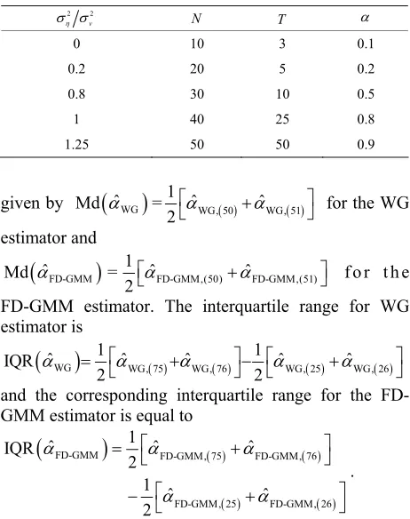
Table 1. Monte carlo designs.

2 2

v



  N T 

0 10 3 0.1

0.2 20 5 0.2

0.8 30 10 0.5

1 40 25 0.8

1.25 50 50 0.9

given by Md



ˆ_WG



=1 ˆ_{WG, 50 } ˆ_{WG, 51 }

2   for the WG estimator and



ˆFD-GMM



Md  =1 ˆFD-GMM,(50) ˆFD-GMM,(51)

2   f o r t h e FD-GMM estimator. The interquartile range for WG estimator is



WG



WG, 75_{ } WG, 76_{ } WG, 25_{ } WG, 26_{ }

1 1

ˆ ˆ ˆ ˆ ˆ

IQR

2 2

 _  _ _  _ 

   

and the corresponding interquartile range for the FD- GMM estimator is equal to





   

   

FD-GMM FD-GMM, 75 FD-GMM, 76

FD-GMM, 25 FD-GMM, 26 1

ˆ ˆ ˆ

IQR

2

1 ˆ ˆ

2

  

 

 

 _  _

 

 _  _

.

[8] computed the asymptotic approximations to the bias given by



1



T and



1



N for WG and FD-GMM estimators, respectively.

6. Results and Discussion

We report the Monte Carlo simulations on the WG and FD-GMM estimators for various combinations of values of N and T, and relatively wide range of values for

 and 2 2

 

  . The main focus of the analysis is on the bias of the WG and FD-GMM estimators as the number of cross-section dimension and the number of time dimension changes. The change in bias as the true value of the coefficient parameter

N T

 varies is also shown. The effect of the variance ratio between the individual effect and the random disturbance on the bias of the two estimators is explored.

6.1. Effect of the Sample Size on the Bias The marginal effect of varying the cross-section dimen-sion and the time dimension T are presented separately. The joint effect of and T is also pre-sented as [8] emphasized that the asymptotic bias of the DPD estimators depend on the relative rates of increase of and T.

N

N

N

In theory, the cross-section dimension has no ef-fect on the bias of the WG estimator. This is confirmed

in the simulation exercise, where the bias of WG estima-tor is relatively constant as varies, given that is fixed. On the other hand, the theory is that the FD-GMM estimator has a bias of order

N T

1 N, that is, the bias de-creases as becomes large. This pattern is not per-fectly observed in the simulation. For instance, when the variance ratio

N

2 2 ₁

 

   , only 10 out of the 25 cases have shown the pattern of decreasing bias of the FD-GMM estimates as the number of cross-section di-mension increases. Also, when the variance ratio

2 2 ₀

 

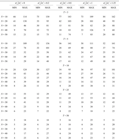
[image:7.595.91.509.230.720.2]

   , only 10 out of the 25 cases have shown the pattern of decrease in bias as increases. A summary of the range of values of bias as percentage of the true parameter value for the FD-GMM estimator focusing on varying the cross-section dimension is presented in Table 2. For a moderate time dimension

N

N

10 T  , we could expect a FD-GMM estimate with a bias from 14% to 47% for N30, from 8% to 39% for N40 and from 6% to 38% of the true value of the coefficient even when N50.

Table 2. Percent bias of ˆFD-GMM.

2 2_0 2 2 _0.2

 

   2 2 _0.8 2 2 ₁

 

   2 2 _1.25

 

  

 

     

MIN MAX MIN MAX MIN MAX MIN MAX MIN MAX

T = 3

N= 10 66 114 75 130 77 183 73 189 84 162

N = 20 41 138 33 95 62 103 28 101 48 95

N= 30 14 46 30 81 15 81 38 82 28 88

N = 40 9 70 12 72 10 83 33 126 9 68

N = 50 15 21 15 75 11 74 7 85 20 88

T = 5

N= 10 53 109 52 136 56 141 58 111 52 161

N= 20 27 74 33 101 28 69 40 80 37 74

N= 30 22 52 25 50 23 62 24 67 25 59

N= 40 14 59 22 48 16 61 13 67 18 61

N= 50 3 29 14 48 17 61 12 49 18 59

T = 10

N = 10 28 124 30 127 34 95 36 97 32 101

N= 20 18 83 21 44 19 55 27 39 26 71

N= 30 14 32 15 27 16 34 18 47 19 43

N= 40 8 39 10 29 11 32 14 32 11 34

N = 50 8 26 11 38 8 28 10 30 6 31

T = 25

N= 10 12 55 12 29 13 49 13 37 12 41

N= 20 11 42 13 55 11 43 13 53 13 44

N= 30 9 41 11 28 11 29 10 28 12 45

N= 40 6 23 9 54 9 34 8 30 7 27

N= 50 6 23 7 22 8 22 7 18 5 25

T = 50

N= 10 5 18 6 18 5 16 5 25 5 31

N = 20 5 24 6 24 5 18 6 20 6 20

N= 30 5 23 5 27 6 22 5 21 5 22

N= 40 5 17 6 27 6 24 6 22 6 20

L. A. SANTOS ET AL. 65

The time dimension affects the bias of the WG es-timator. The WG estimator has bias of order T 1T, that is, as becomes larger, the WG bias becomes smaller. This is also observed in the simulation. As expected, as increases from 3 to 50, the bias reduces tremendously within acceptable levels as T is nearing 50. This pattern is implied by the increase of the magnitude of the medi-ans as becomes larger.

T T

T

The FD-GMM estimator is known to be affected by the cross-section dimension N, and the order of bias is 1 N and does not involve T 8] noted that consistency of the FD-GMM estimator requires





. [

2 logT N0

and T s mean he bias

of the FD-GMM estimator does not depend on N alone but also T. he FD-GMM esti ates in the simulation exercise illustrate the decrease in bias as the time dimen-sion increases, most specially for 0.5

where hi s that t

m N 

T

. T

  . Also, from

Table 2, a FD-GMM estimate is within 6% to 12 f the true value, when T 10

7% o  , within 6% to 55% f the true value when T 25

o  and within 4% to 27% of the true value of the coefficient, implying the magnitude of

-GMM bias

FD decreases as T increases.

T

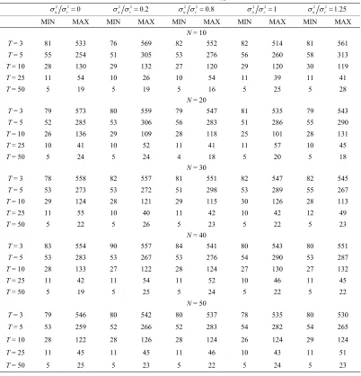
A summary of the range of values of bias as percentage of the true parameter value for the WG estimator with varying time dimension is presented in Table 3. For a small cross-section dimension , one could ex-pect a WG estimate with a bias from 27% to 132% for N 10



10

T  , from 10% to 54% for and from 5% to 28% of the true value of the coefficient when 25



T

[image:8.595.98.500.307.725.2]

50 T  . Even for large cross-section dimension, say N 50, the WG estimates have similar range of percent bias as those estimate when N 10. This indeed shows that there is notable decrease in the bias of WG estimates as in-creases whatever the value of N. T Table 3. Percent bias of ˆWG.

2 2 ₀

 

   2 _2_0.2

 

 2 2 _0.8

 

   2 2 ₁

 

   2 2 _1.25

 

  

MIN MAX MIN MAX MIN MAX MIN MAX MIN MAX

N = 10

T 3 81 533 76 569 82 552 82 514 81 561

N = 20

T 3 79 573 80 559 79 547 81 535 79 543

N = 30

T 3 78 558 82 557 81 551 82 547 82 545

N = 40

T 3 83 554 90 557 84 541 80 543 80 551

N = 50

T 3 79 546 80 542 80 537 78 535 80 530

=

T= 5 55 254 51 305 53 276 56 260 58 313

T= 10 28 130 29 132 27 120 29 120 30 119

T= 25 11 54 10 26 10 54 11 39 11 41

T= 50 5 19 5 19 5 16 5 25 5 28

=

T= 5 52 285 53 306 56 283 51 286 55 290

T= 10 26 136 29 109 28 118 25 101 28 131

T= 25 10 41 10 52 11 41 11 57 10 45

T= 50 5 24 5 24 4 18 5 20 5 18

=

T= 5 53 273 53 272 51 298 53 289 55 267

T= 10 29 124 28 121 29 115 30 126 28 113

T= 25 11 55 10 40 11 42 10 42 12 49

T= 50 5 22 5 26 5 23 5 22 5 23

=

T= 5 53 283 53 267 53 276 54 290 53 287

T= 10 28 133 27 122 28 124 27 130 27 132

T= 25 11 42 11 54 11 52 10 46 11 45

T= 50 5 19 5 25 5 24 5 22 5 22

=

T= 5 53 259 52 266 52 283 54 282 54 265

T= 10 28 122 28 126 28 124 26 124 29 124

T= 25 11 45 11 45 11 46 10 43 11 51

It is interesting to note that the relationship een ia

betw b s and the sample size represented by the pair (N,T) also takes into account the relative rates of increase of N with respect to T for the WG estimator and T with respect to N for the FD-GMM estimators. When we have a square panel, that is when the sample size is either, (N10,T10) or (N50,T 50), the WG estimates and GMM estimates are almost the same. The similarity of the WG estimates to the GMM estimates is also seen for an almost square panel, such as (N20,T 25), (N30,T 25), and N = 40, T = 50. This confirms the theory of [8] that the asymptotic bias of WG and FD-GMM are the same when N T , we confirmed here to be also true for moderate samples and even small samples. When T 50, regardless of the size of N, the value of WG estimates are similar to the value of FD-GMM estimates. This is attributed to the fact that in the previously stated scenario, the time-series dimension is always greater than or equal to the cross-section dimension, in this case the workable for-mula for FD-GMM whenever tN is almost identical to the WG formula.

.2. Effect of Para

6 meter Values on the Bias y has The first-order DPD model considered in this stud three parameters, but we focused only on the coefficient of the lagged dependent variable (). The two other parameters are the variances of the one-way random ef-fects error component, namely the variance of the indi-vidual effect 2



 and the variance of the random dis-turbance 2



 . Instead of analyzing the effect of 2



 and 2



 separately, we focus on the variance ratio 2 2

 

  . Both the WG and FD-GMM estimators are do ward

sed, that is, the estimates are smaller than wn

bia the true

value of the coefficient parameter  . As shown by [2] for WG estimator, the bias decreases as  increases. This is true for both the WG and FD-GMM estimators as illustrated in the study. Also, one may think that the per-cent bias will increase as we decrease the value of  , since the smaller the value of the denominator the larger the fraction becomes. This is confirmed in the results of simulation, the FD-GMM bias decrease as T increase provided that  is large.

The exact distribution of WG estimator is said to be invariant to bo the varianceth of the individual effect 2





and the variance of the random disturbance 2



 , while the distribution of the FD-GMM estimator is invariant only to the variance ratio 2 2

 

  , see [8]. In the simula-tion exercise, varying the variance ratio does not show sizeable changes on the bias, when the sample size



N T,



and the value of the parameter coefficient 

are fixed.

WG and FD-GMM Estimators We compar

6.3. Other Asymptotic and Finite Sample Properties of

betw

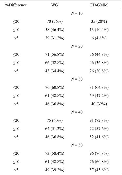
ported in Table 4. The following asymptotic properties: e the median of the estimators to the ap-proximate bias values computed by [8]. Percent different een the computed bias and the approximate bias are re

(a) when T N , the asymptotic bias of GMM is smaller than the WG bias, (b) when T N, the expres-sion for the two asymptotic biases are equal and (c) when

0

N T , the asymptotic bias in the WG estimator dis-appears, der y Alvarez and Arellano (2003) still hold for smaller samples considered study. The findings of [7] that the WG is more efficient than GMM

ported by the simulation study. Since the bias of WG estimator does not depend on N, the values are similar, that is, the number of WG estimates with percent difference values less than 5% is almost the same for different values of N. On the other hand, percent dif-ference of FD-GMM estimate increases with N. The asymptotic approximation of [8] performs well for

40

[image:9.595.309.540.393.724.2]

N , since 72.8% of the MC medians of FD-GMM estimates are within % of the approximated value.

Table 4. Percent difference of bias estimates from asymp-ses.

%Difference WG FD-GMM

ived b

in this

is also sup

20

totic bia

N = 10

<20 70 (56%) 35 (28%)

<10 58 )

<5 39 (31.2%) 6 (4.8%)

N = 20

(46.4% 13 (10.4%)

<20 71 (56.8%) 56 (44.8%)

<10 66 (52.8%) 4

<5 43 (34.4%) 26 (20.8%)

N = 30

6 (36.8%)

<20 76 (60.8%) 81 (64.8%)

<10 61 (48.8%) 59 (47.2%)

<5 46 (36.8%) 40 (32%)

N = 40

<20 75 (60%) 91 (72.8%)

<10 64 (51.2%) 72 (57.6%)

<5 46 (36.8%) 52 (41.6%)

N = 50

<20 73 (58.4%) 96 (76.8%)

<10 61 (48.8%) 76 (60.8%)

L. A. SANTOS ET AL. 67

The of FD-G aller than t WG

estim that is 71 t of 125 c this

pattern ote that 6 e cases ha up

d the othe e the set-u

bias MM is sm he bias of

ates, . N

(56.8%) ou 0% of th

ases follow ve the set-T N

int

, an r 40% hav p T N. It is eresting to note that only when the variance of the individual effect 2



 equal to zero, we see that majority, that is, 20 out of the 25 cases considered have bias of

M less than the bias of WG. On the other hand, when 2 ₀



  , half of the cases have bias of FD-GMM smaller than bias WG and the other half have bias of WG less than or equal to bias of FD-GMM. The cases where bias of WG is less than or equal to the bias of FD-GM timates have moderate to large T , but when T 10, the bias of WG is smaller and closer to the FD-GMM bias only when

FD-GM

of

M es

 is at least 0.5. Spe-cifically, bias of WG is close to bias of FD-GMM for square panels where 0.5 and for T 25.

We nalyzed moderately-sized cross-section

di-mension, i.e., N30. This 0% the 125 ca

allows for 8 of

ses to have TN and the other 20% are designs where T N. pect that more percentage of FD- GMM estimates maller bias than WG estimates as compar where the cross-dimension size is small. There are 90 (72%) of the 125 cases where bias of FD-GMM is smaller than the bias of WG. The other 35 (28%) cases have either large time-dimension, that is

50 T

We ex have s ed to

 or larger value for the coefficient parameter, which is  0.8. This is intuitively true, since when

50

T  , N T and the bias of WG is expected to be less than of FD-GMM. For moderately-sized mension, about 73% of the FD-GMM estimates have smaller bias than their WG counterpart and the other 27% have designs where the time dimen-sion is large or the value of the coefficient of parameter is close to one.

Some 80% of the 125 cases have designs where T < N also a

the bias cross-section di

WG

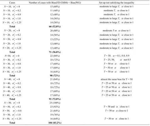
[image:10.595.62.540.323.726.2]

Cases Numbe tisfying the inequality

Table 5. Comparison of bias of and FD-GMM estimates.

r of cases with Bias(FD-GMM) < Bias(WG) Set-up not sa

N = 10, 2 ₀ large T,



  15 (60%) moderate to close to 1

N = 10, 2



 0.2 11 (44%) moderate T, close to 1

N = 10, 2 _0.8



  12 (48%) moderate T, close to 1

N = 10, 2 _1.0



  14 (56%) moderate to large , T close to 1

mo T

N = 10, _2_1.25

 14 (56%) derate to large , close to 1

l 66

Tota (52.8%)

N = 20, 2 ₀



  20 (80%) moderate T or clo

N = 2 moderate to larg T,

se to 1 0, 2



 0.2 14 (56%) e close to 1

mo ,

N = 20, _2_0.8

 13 (52%) derate to large T close to 1

N = 20, _2_1.0

 12 (48%) moderate to large T, close to 1

N = 20, _2_1.25

 12 (48%) moderate to large T, close to 1

Total 71 (56.8%)

N=30, 2 ₀



  22 (88%) T = 50. = 0.1, 8, 0.9 0.

N = 30, 2 T = 25,



 0.2 18 (72%) 50,  not 0.5

N = 30, _2_0.8

 17 (68%) T = 50 or  close to 1

N = 30, _2_1.0

 17 (68%) T = 50 or  close to 1

N = 30, _2_1.25

 16 (64%) T = 50 or  close to 1

Total 90

alm e 0

N = 4 T = 25 or 50 or

(72%)

N = 40, 2 ₀



 

0.2

21 (84%) ost the sam bias for T = 5

0, 2



  18 (72%)  close to 1

N = 40, 2 _0.8



  18 (72%) T = 25 or 50 or  close to 1

N = 40, 2 _1.0



  17 (68%) T = 25 or 50 or  close to 1

N = 40, 2 _1.25



  17 (68%) T = 25 or 50 or  close to 1

Total 91

2

N = 5 T = 50 and

(72.8%)

N = 50, 0 0.2

25 (100%) 0, 2



  23 (92%)  close to 1

N = 50, 2 _0.8 T = 50 or



  21 (84%) close to 1

N = 50, 2 _1.0



  19 (76%)

N = 50, 2 _1.25



  16 (64%) T = 50 or  close to 1

an of the cases come from squa that is, expect that most of th

esti-rate size cross-sectio i are 105 (84%) cases where IQR of WG is less than IQR of FD-GMM. The strongest evidence that the WG estimator has sma riabilit -GMM is seen in the sum-ma ble 6, articularly, 11 ) of the 125

cases ha of WG smaller tha D-GMM.

h

eir

d 20% re panel,

50. We

N T  e FD-GMM

[image:11.595.57.291.273.718.2]

mates have smaller bias than the WG estimates and when square panels are considered the biases are the same. There are 104 (83.2%) of the 125 cases considered has FD-GMM bias smaller than their WG counterpart. The other 21 (16.8%) cases have designs where the time di-mension is large, that is, T 50 and the coefficient parameter is close to one, that is,  0.8 or 0.9.

Table 6 summarizes comparison of the variability of WG and FD-GMM estimates as easured by the inter-quartile range (IQR). The WG es ates generall

m

tim y have

less variability than FD-GMM estimates, for the

mode-Table 6. Comparison of variability of WG and FD-GMM estimates.

Cases Interquartile Range (WG) < Interquartile _{Range (GMM)}

N = 10, 2 ₀



  21 (84%)

N = 1

tal 97

N = 2

tal 111

N = 3

tal 105

N = 4

tal 112

N = 5

Total 113 (90.4%)

0, 2



 0.2 18 (72%)

N = 10, 2 _0.8



  20 (80%)

N = 10, 2 _1.0



  20 (80%)

N = 10, 2 _1.25



  18 (72%)

To (77.6%)

N = 20, 2 ₀



  22 (88%)

0, 2



  2

0.2 22 (88%)

N = 20, 0.8 23 (92%)

N = 20, 2 _1.0



  23 (92%)

N = 20, 2 _1.25



  21 (84%)

To (88.8%)

N = 30, 2 ₀



  17 (68%)

0, 2



 0.2 20 (80%)

N = 30, 2 _0.8



  24 (96%)

N = 30, 2 _1.0



  22 (88%)

N = 30, 2 _1.25



  22 (88%)

To (84%)

N = 40, 2 ₀



  22 (88%)

0, 2



  2

0.2 22 (88%)

N = 40, _0.8 20 (80%)

N = 40, 2 _1.0



  24 (96%)

N = 40, 2 _1.25



  24 (96%)

To (89.6%)

N = 50, 2 ₀



  24 (96%)

0, 2



  2

0.2 23 (92%)

N = 50, 0.8 23 (92%)

N = 50, 2 _1.0



  22 (88%)

N = 50, 2 _1.25



  21 (84%)

n dimens on. There

ller va y than FD

ry of Ta p 3 (90.4%

ve IQR n IQR of F

6.4. Comparison of Bootstrapped DPD and

Conventional DPD Estimators

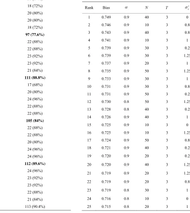
To be able to assess the benefits from boostrapping the WG and GMM estimators, we identified settings in the mulation scenarios where they yield the largest bias. si

We report in Tables 7 and 8 the top 25 of estimates wit the largest bias for both WG and GMM, together with

[image:11.595.146.523.304.726.2]

respective design specifications. th

Table 7. 25 Largest bias of WG estimates and their design specifications.

Rank Bias  N T 2





1 0.749 0.9 40 3 0

2 0.746 0.9 10 3 0.8

3 0.743 0.9 40 3 0.8

4 0.741 0.9 10 3 1

0. 30 3 0.2

1

1

1

25 0.715 0.8 20 3 1

5 0.739 9

6 0.739 0.9 30 3 .25

7 0.737 0.9 20 3 1

8 0.735 0.9 50 3 1.25

9 0.733 0.9 30 3 1

10 0.731 0.9 30 3 0.8

11 0.731 0.9 50 3 0.2

12 0.730 0.8 50 3 .25

13 0.728 0.8 40 3 0.2

14 0.726 0.9 40 3 1

15 0.725 0.9 10 3 0

16 0.725 0.9 10 3 1.25

17 0.724 0.9 50 3 0.8

18 0.721 0.9 40 3 0.2

19 0.720 0.9 20 3 0.2

20 0.720 0.9 40 3 .25

21 0.719 0.9 20 3 1.25

22 0.719 0.9 20 3 0.8

23 0.719 0.8 30 3 1

L. A. SANTOS ET AL. 69

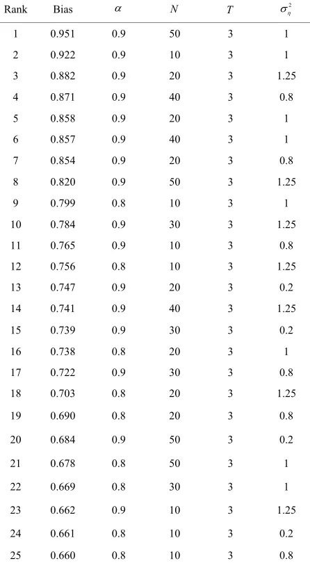
Ta 8. 2 t of FD M est ates an design spe tions.

Rank Bias ble 5 Larges

cifica

bias -GM im d their

 N T 2





1 0.951 0.9 50 3 1

2 0.922 0.9 10 3 1

3 0.882 0.9 20 3 1.25

4 0.871 0.9 40 3 0.8

0.9 20 3 1

0.

10

11 0. 0.

12

13 0.

14 5 0.858

6 0.857 0.9 40 3 1

7 0.854 0.9 20 3 8

8 0.820 0.9 50 3 1.25

9 0.799 0.8 10 3 1

0.784 0.9 30 3 1.25

765 0.9 10 3 8

0.756 0.8 10 3 1.25

747 0.9 20 3 0.2

0.741 0.9 40 3 1.25

15 0.739 0.9 30 3 0.2

16 0.738 0.8 20 3 1

17 0.722 0.9 30 3 0.8

18 0.703 0.8 20 3 1.25

19 0.690 0.8 20 3 0.8

20 0.684 0.9 50 3 0.2

21 0.678 0.8 50 3 1

22 0.669 0.8 30 3 1

23 0.662 0.9 10 3 1.25

24 0.661 0.8 10 3 0.2

25 0.660 0.8 10 3 0.8

or bia the W estimator is

The der of s of G 1T and

therefore, as increases the reases. The order

of s o ator is

T bias dec

bia f the GMM estim 1 N and thus, as N he

h

first

in ses as eases. rms bi

worst WG ates came from designs wit e small tim di sion. s is c ruent to the

eoretical p rties of the WG estimator, but at qu

crea , the bi

e rope

decr In te of the as, t and GMM estim

men v

th

ry Thi ong

ite surprising for GMM estimator. When T3 , FD-GMM estimator uses only one instrument and thus equivalent to the IV estimator, less appealing than the GMM estimators. Moreover, the FD-GMM estimator when T 3, does not show a decrease in bias as N becomes larger.

It is known that the bias of WG estimator increases with the coefficient parameter  , see [2] and [7]. s simulation exercise, all the WG and GMM worst

esti-mates came from designs with large

In thi

, see Table 9. As the autoregression component of the model becomes nearly n ationary, both WG and FD-GMM estimat can suffer tremend

onst es

ously.

[image:12.595.60.283.109.514.2]

el

Table 9. Monte carlo designs yi ding worst estimates (33 parameter combinations).

Design  N T 2



 2

v



1 0.8 10 3 0 1

2 0.8 10 3

3

3

0.2 1

1 1

0. 10 1.25 1

0.

1

1

1.

1.

1.

3 0.8 10 3 0.8 1

4 0.8 10

5 8

6 0.8 20 3 8 1

7 0.8 20 3 1 1

8 0.8 20 3 1.25 1

9 0.8 30 3 1 1

10 0.8 40 3 0.2 1

11 0.8 50 3 1 1

12 0.8 50 3 .25 1

13 0.9 10 3 0 1

14 0.9 10 3 0.8 1

15 0.9 10 3 1 1

16 0.9 10 3 .25 1

17 0.9 20 3 0.2 1

18 0.9 20 3 0.8 1

19 0.9 20 3 1 1

20 0.9 20 3 25 1

21 0.9 30 3 0.2 1

22 0.9 30 3 0.8 1

23 0.9 30 3 1 1

24 0.9 30 3 25 1

25 0.9 40 3 0 1

26 0.9 40 3 0.2 1

27 0.9 40 3 0.8 1

28 0.9 40 3 1 1

29 0.9 40 3 1.25 1

30 0.9 50 3 0.2 1

31 0.9 50 3 0.8 1

32 0.9 50 3 1 1

[image:12.595.305.538.169.718.2]

T riances of t ndividual effe r the orst

GMM estim are m act out of th

desig s consid ha and 21 ut of t 25

cas onsid have The variances the

ind e ts of st WG ates are

similar.

W e ine design for th larges ias

of

) both ology is

rror for the original estimators WG and FD- G

(b)

ev.

he va he i ct fo w

ates ered

ostly large ve

, in f 15 o

e 25 he

n 2 ₁



  2 _0.8

  25 w

es c ered  . of

ividual ffec the or estim

hen w comb the s e 25 t b

WG and 25 largest bias of GMM, they have 17 com-mon designs, thus 33 designs in Table 9 represent the worst estimate (largest bias from WG and GMM.

The bootstrap method used for these 33 de-signs. The bias, standard deviation and the root mean square e

MM together with the bootstrap estimators WGb and FD-GMM b are presented in Tables10(a)-(e).

Tables 10. (a) Estimates for = 0.8, N = 10, 20; (b) Esti-mates for = 0.8, N = 30, 40, 50; (c) Estimates for = 0.9, N = 10, 20; (d) Estimates for = 0.9, N = 30, 40; (e) Esti-mates for = 0.9, N = 50.

(a)

Design Bias Std. Dev. MSE

1 WG 0.716 0.221 0.561

Gb 0.751 0.117 0.

FD-GMM 0.596 0.662 0.793 FD-GMMb 0

W 578

.701 0.137 0.510

2 WG 0.705 0.215 0.543

WGb MM MMb

MMb 4*w m

5*w m

1.264 0.259 1.665

FD-G

FD-G

0.661 1.226

0.692 1.004

0.916 2.511

3 WG 0.678 0.200 0.500

WGb 1.196 0.162 1.457

FD-GMM 0.660 0.905 1.255

g,gm

FD-G 1.291 0.699 2.156

WG 0.708 0.189 0.537

WGb 0.489 0.063 0.243

FD-GMM MMb

0.799 1.242 2.181

g,gm

FD-G 0.518 0.261 0.337

WG 0.713 0.215 0.555

WGb 0.706 0.019 0.498

FD-GMM MMb

0.756 0.744 1.125

FD-G 0.705 0.085 0.504

6 WG 0.684 0.167 0.496

WGb 0.965 0.036 0.933

FD-GMM MMb

0.690 1.062 1.604

FD-G 0.966 0.253 0.997

7 WG 0.715 0.162 0.537

WGb 0.889 0.061 0.794

FD-GMM MMb

0.738 1.334 2.324

FD-G 0.865 0.264 0.819

8 WG 0.674 0.127 0.470

WGb 0.990 0.052 0.982

FD-FD-GMM GMMb

0.703 0.977

0.864 0.223

1.241 1.004

Bias Std. D MSE

9 WG 0.719 0.127 0.533

WGb 0.964 1

MM 5

b 4

6

WGb 0.768 0.076 0.595

FD-G M MMb

11*w gmm

MMb 1

MMb

0.05 0.932

FD-G 0.669 0.55 0.756

FD-GMM 0.936 0.16 0.902

10 WG 0.728 0.09 0.539

M 0.448 0.765 0.786

FD-G 0.829 0.463 0.901

g, _{WG 0.698 0.09 0.495}

WGb 0.437 0.006 0.191

FD-GMM 0.678 0.688 0.933

FD-G 0.433 0.021 0.188

2 WG 0.73 0.091 0.541

WGb 1.014 0.016 1.029

FD-GMM 0.502 0.867 1.004

FD-G 1.007 0.080 1.021

(c)

S .

Bias td. Dev MSE

13 WG 0.725 0.254 0.590

WGb 1.468

14*w _{WG 0.746 0.249 0.619}

WGb 0.618 0.018 0.382

FD-GM MMb 15* gmm

MMb 1

0.243 2.215

FD-GMM 0.614 1.119 1.629

g,gmm

FD-GMMb 1.230 0.443 1.710

M 0.765 0.785 1.201

FD-G 0.614 0.029 0.377

wg, _{WG 0.741 0.217 0.596}

WGb 0.216 0.058 0.050

FD-GMM 0.922 0.950 1.753

FD-G 0.203 0.086 0.049

6 WG

WGb

0.725 1.088

0.254 0.026

0.590 1.184

FD-GMM 0.662 0.787 1.058

FD-GMMb 1.075 0.168 1.183

17*wg,gmm _{WG 0.720 0.167 0.546}

WGb 0.396 0.022 0.158

FD-GMM 0.747 0.760 1.136

FD-GMMb 0.393 0.072 0.160

18 WG 0.719 0.157 0.542

WGb 0.864 0.055 0.750

FD-GMM 0.854 0.738 1.274

FD-GMMb 0.869 0.204 0.797

19 WG 0.737 0.172 0.573

WGb 1.150 0.030 1.324

FD-GMM 0.858 0.832 1.428

FD-GMMb 1.144 0.069 1.314

20 WG 0.719 0.163 0.544

WGb 1.316 0.026 1.733

FD-GMM 0.882 0.808 1.431