Optimizing single mode collection from pointlike sources of single photons with adaptive optics

Optimizing single-mode collection from

pointlike sources of single photons with

adaptive optics

A

D. H

,

D

H

,

J

N

,

M

G

,

A

B

,

U

P

,

D

S

,

C

S

,

M

K

,

S

H

,

J

W

,

J

L

,

W

Z

,

P

G. K

1_{University of Illinois at Urbana-Champaign, Department of Physics, 1110 West Green Street, Urbana, IL}

61801-3080, United States of America

2_{Universidad San Francisco de Quito, Av. Diego de Robles y Vìa Interoceánica, Riobamba, Ecuador} 3_{Norman Bridge Laboratory of Physics MC12-33, California Institute of Technology, Pasadena, California}

91125, USA

4_{University of Michigan, Department of Physics, 450 Church Street, Ann Arbor, MI 48109-1040, United}

States of America

5_{Technische Physik and Wilhelm-Conrad-Röntgen Research Center for Complex Material Sytems,}

University of Würzburg, 97074 Würzburg, Germany

6_{SUPA, School of Physics and Astronomy, University of St. Andrews, St. Andrews, KY16 9SS, United}

Kingdom

*_{[email protected]}

Abstract: The collection efficiency of light from a point-like emitter may be extremely poor due to aberrations induced by collection optics and the emission distribution of the source. Analyzing the aberrant wavefront (e.g., with a Shack-Hartmann sensor) and correcting accordingly can be infeasible on the single-photon level. We present a technique that uses a genetic algorithm to control a deformable mirror for correcting wavefront aberrations in single-photon signals from point emitters. We apply our technique to both a simulated point source and a real InAs quantum dot, achieving coupling increases of up to 50% and automatic reduction of system drift.

© 2017 Optical Society of America

OCIS codes:(110.1080) Active or adaptive optics; (270.0270) Quantum optics.

References and links

1. J. D. Sterk, L. Luo, T. a. Manning, P. Maunz, and C. Monroe, “Photon collection from a trapped ion-cavity system,” Phys. Rev. A85, 062308 (2012).

2. R. Noek, G. Vrijsen, D. Gaultney, E. Mount, T. Kim, P. Maunz, and J. Kim, “High Speed, High Fidelity Detection of an Atomic Hyperfine Qubit,” Opt. Lett.38, 4 (2013).

3. W. B. Gao, a. Imamoglu, H. Bernien, and R. Hanson, “Coherent manipulation, measurement and entanglement of individual solid-state spins using optical fields,” Nat. Photonics9, 363–373 (2015).

4. K. H. Madsen, S. Ates, J. Liu, A. Javadi, S. M. Albrecht, I. Yeo, S. Stobbe, and P. Lodahl, “Efficient out-coupling of high-purity single photons from a coherent quantum dot in a photonic-crystal cavity,” Phys. Rev. B90, 155303

(2014).

5. M. Arcari, I. Söllner, A. Javadi, S. Lindskov Hansen, S. Mahmoodian, J. Liu, H. Thyrrestrup, E. H. Lee, J. D. Song, S. Stobbe, and P. Lodahl, “Near-Unity Coupling Efficiency of a Quantum Emitter to a Photonic Crystal Waveguide,” Phys. Rev. Lett.113, 1–5 (2014).

6. G. M. Akselrod, C. Argyropoulos, T. B. Hoang, C. Ciracì, C. Fang, J. Huang, D. R. Smith, and M. H. Mikkelsen, “Probing the mechanisms of large Purcell enhancement in plasmonic nanoantennas,” Nat. Photonics8, 835–840

(2014).

7. N. Somaschi, V. Giesz, L. De Santis, J. C. Loredo, M. P. Almeida, G. Hornecker, S. L. Portalupi, T. Grange, C. Anton, J. Demory, C. Gomez, I. Sagnes, N. D. L. Kimura, A. Lemaitre, A. Auffeves, A. G. White, L. Lanco, and P. Senellart, “Near optimal single photon sources in the solid state,” Nat. Photonics10, 1–6 (2015).

9. A. Tiranov, P. C. Strassmann, J. Lavoie, N. Brunner, M. Huber, V. B. Verma, S. W. Nam, R. P. Mirin, A. E. Lita, F. Marsili, M. Afzelius, F. Bussières, and N. Gisin, “Temporal multimode storage of entangled photon pairs,” Phys. Rev. Lett.117, 240506 (2016).

10. G. N. M. Tabia, “Recursive multiport schemes for implementing quantum algorithms with photonic integrated circuits,” Phys. Rev. A93, 012323 (2016).

11. M. L. Plett, P. R. Barbier, and D. W. Rush, “Compact adaptive optical system based on blind optimization and a micromachined membrane deformable mirror.” Appl. Optics40, 327–330 (2001).

12. A. Courteville, “Optimization of single-mode fiber coupling efficiency with an adaptive membrane mirror,” Opt. Eng.

41, 1073 (2002).

13. P. Villoresi, S. Bonora, M. Pascolini, L. Poletto, G. Tondello, C. Vozzi, M. Nisoli, G. Sansone, S. Stagira, and S. De Silvestri, “Optimization of high-order harmonic generation by adaptive control of a sub-10-fs pulse wave front.” Opt. Lett.29, 207–209 (2004).

14. C. Bonato, S. Bonora, A. Chiuri, P. Mataloni, G. Milani, G. Vallone, and P. Villoresi, “Phase control of a path-entangled photon state by a deformable membrane mirror,” J. Opt. Soc. Am. B27(2010).

15. M. Minozzi, S. Bonora, a. V. Sergienko, G. Vallone, and P. Villoresi, “Optimization of two-photon wave function in parametric down conversion by adaptive optics control of the pump radiation.” Opt. Lett.38, 489–491 (2013).

16. V. N. Mahajan, “Strehl ratio of a Gaussian beam.” J. Opt. Soc. Am. A22, 1824–1833 (2005).

17. A. P. Burgers, J. R. Schaibley, and D. G. Steel, “Entanglement and Quantum Optics with Quantum Dots,” in “From Atomic to Mesoscale,” (World Scientific, 2015), pp. 103–120.

18. W. B. Gao, P. Fallahi, E. Togan, J. Miguel-Sanchez, and A. Imamoglu, “Observation of entanglement between a quantum dot spin and a single photon,” Nature491, 426–430 (2012).

19. K. De Greve, L. Yu, P. L. McMahon, J. S. Pelc, C. M. Natarajan, N. Y. Kim, E. Abe, S. Maier, C. Schneider, M. Kamp, S. Höfling, R. H. Hadfield, A. Forchel, M. M. Fejer, and Y. Yamamoto, “Quantum-dot spinâĂŞphoton entanglement via frequency downconversion to telecom wavelength,” Nature491, 421–425 (2012).

20. J. R. Schaibley, A. P. Burgers, G. A. McCracken, L.-M. Duan, P. R. Berman, D. G. Steel, A. S. Bracker, D. Gammon, and L. J. Sham, “Demonstration of quantum entanglement between a single electron spin confined to an inas quantum dot and a photon,” Phys. Rev. Lett.110, 167401 (2013).

21. B. Hensen, H. Bernien, A. E. Dréau, A. Reiserer, N. Kalb, M. S. Blok, J. Ruitenberg, R. F. L. Vermeulen, R. N. Schouten, C. Abellán, W. Amaya, V. Pruneri, M. W. Mitchell, M. Markham, D. J. Twitchen, D. Elkouss, S. Wehner, T. H. Taminiau, and R. Hanson, “Loophole-free Bell inequality violation using electron spins separated by 1.3 kilometres,” Nature526, 682–686 (2015).

22. J. Enderlein, “Theoretical study of detection of a dipole emitter through an objective with high numerical aperture,” Opt. Lett.25, 634–636 (2000).

23. R. Maiwald, A. Golla, M. Fischer, M. Bader, S. Heugel, B. Chalopin, M. Sondermann, and G. Leuchs, “Collecting more than half the fluorescence photons from a single ion,” Phys. Rev. A86, 043431 (2012).

1. Introduction

Efficient collection of photons emitted from point-like sources (e.g., trapped ions [1, 2], nitrogen-vacancy centers [3], quantum dots [3, 4], etc.) is often critical for the interrogation of single quantum systems and the efficient realization of quantum computing and communication protocols. Collection optics often introduce significant wavefront aberrations due to the clipping and focusing of collected light from an effective point source. Due to these aberrations and a small collection solid angle, coupling of the light emitted by an interrogated quantum system into a single-mode optical fiber (SMF) – the most natural way to connect separate quantum systems – may be extremely inefficient, despite the fact that the light is emitted into a single spatial mode (e.g., a dipole radiation mode). Recent work in producing radiation from pointlike objects in the desired mode has been quite successful using microcavities and antennae matched to the source [5–7]; however, they may be difficult to implement in existing experimental setups in general. Other purely optical approaches have proven successful [8], but are designed for isotropic sources. Note that as photon emitters are contemplated for use in multi-photon quantum information processing applications, e.g., multi-mode quantum repeater networks [9] or demonstrations of photonic integrated circuit based quantum algorithms [10], even modest improvements in coupling efficiency can lead to large net enhancements – especially in multiphoton experiments.

systems, photonic circuitry, etc.). AO is effective for optimizing spatial modes for coupling applications [11,12] and nonlinear optics [13]; however, AO can be difficult in the low-intensity limit, where wavefront measurements are unreliable and photon count fluctuations can thwart traditional gradient methods of system optimization. In this regime, AO must be performed entirely at the single-photon level [14, 15]. We have developed a “drop-in” AO-enhanced collection system that incorporates a novel noise-resistant genetic algorithm to optimize the shape of a deformable mirror for collection of single photons from a point-like emitter into a single-mode optical fiber (SMF) (although we use a SMF as the most common photonic transfer element, our techniques should also work in a large variety of other applications, e.g., enhanced coupling to/from waveguides, plasmonic devices, nano-antennas, etc.). We have tested our system extensively with a simulated point source (directing light through a sub-wavelength aperture) as well as with actual quantum dot photon emitters, and observed significant enhancements in both cases. After describing the genetic algorithm strategy we will present the results of optimizing collection from a sub-wavelength pinhole and from an InAs quantum dot.

2. Genetic Algorithm

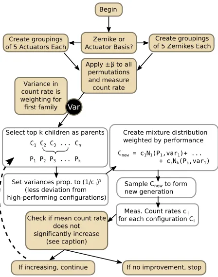
We control the 69 independent electromechanical actuators of a deformable mirror (Alpao DM69) using an in-house designed genetic algorithm specially suited for AO applications with single photons [Fig. 1]. Our algorithm generates random mirror shapes based on previous configurations and weighted by the performance of the generating families; the algorithm first estimates the effect of deforming the mirror on the measured signal (e.g., photon counts coupled into single-mode fiber per second) by computing the count-rate variance observed while randomly permuting subsets of the basis elements. Basis elements may be the full 69 actuators or the 30 lowest-order Zernike polynomials (e.g., tilt, focus, coma, etc.) created over the 69-actuator space of the mirror surface, the choice of which leads to changes in optimization behavior (discussed below). “Child” shapes are constructed by randomly weighting all basis elements to form new generations of mirror configurations. After initialization, randomized deformations are then applied to the mirror surface, creating the “children” of the subsequent generation. The count rate for each of these children is compared; the best test deformations in each generation (the new parents) are weighted by performance and then probabilistically combined to form a new generation of mirror deformations. For our tests, generations were comprised of 20 children from 10 parents selected from the previous generation. Over time (of order 100 generations in our tests) the variance in the generated children is lowered, which allows convergence to an optimal mirror shape.

2.1. Detailed Description of Algorithm

Begin

Create groupings of 5 Actuators Each

Create groupings of 5 Zernikes Each Zernike or

Actuator Basis?

Apply ± to all permutations and measure count rate Variance in

count rate is weighting for

rst family

Check if mean count rate does not signi cantly increase

(see caption)

If no improvement, stop Meas. Count rates c i for each con guration Ci

Cnew = c1N1(P1,var1)+ ...

+ ckNk(Pk,var1)

Set variances prop. to (1/c i) (less deviation from high-performing con gurations)

Create mixture distribution weighted by performance

P1 P2 P3 ... Pk Select top k children as parents

C1 C2 C3 ... Cn

Sample Cnew to form new generation Var

Fig. 1. A schematic of the genetic algorithm. The first generation of mirror configurations is pseudo-randomly generated using a sum of gaussian distributions with variances established by the initialization procedure. Each new generation of mirror configurations is created by weighting gaussian random variables centered on each top-performing mirror configuration, according to count rate. An arbitrary number of children may be generated by sampling this mixture gaussian. The variance of the gaussian random variables is reduced in inverse proportion to configuration performance to allow the mirror generations to converge to an optimal solution. The algorithm completes when it is estimated that the mean has not statistically increased for at least 6 generations.

configuration space needed to optimize collection, since more effective (higher variance) basis elements are allowed to contribute heavily to the first generation of mirror configurations.

After initialization, in each generation we choosekfuture parents from the previousnchildren. The nextnchildren are generated by breeding the chosenkparents using the following procedure. LetYt_i be a random vector ofd elements (dbeing dimension of the space, as defined above) representing the test mirror configuration of thei-th parent at time step t. We select the k highest-performing configurations (those resulting in the most photon counts registered leaving the single-mode fiber in a fixed measurement interval) and form the new generationYt+1 by sampling

Yt+1 = k Õ

i=1

ωiN(Yt_i,aiId), (1)

where N(u, σ) is a multivariate normal distribution with mean u and covariance σ, and

space, andγsets the sensitivity of the search on the count rate relative to the estimated maximum. In our tests, we typically usedn=20,k=10,ρ=3.6×10−6, andγ=0.5. These values were influenced by the simulations shown below; however,ρandγare strongly dependent on the experimental setup (very sensitive corrections require smallρto avoid losing all coupling, for example).

The algorithm completes when the statistics of the count rate do not change significantly for several generations. First, we check if the mean count rate for the past 3 generations differs significantly from the mean for the prior 3 generations (comparing 6 generations total). If the mean has not significantly changed, we then take three new generations with twice the measurement time per mirror configuration to reduce fluctuations. If the mean does not change significantly between these three generations, we stop. In each case we consider the statistics of two generations to be significantly different if|xn¯ −y¯n|<0.93

p

2 ¯yn/n, wherexnis the set of the counts from generationxandynis the set of counts from the current generationy(the two-sample Z-test); 0.93 is a parameter that balances the probabilities of either accepting or rejecting convergence erroneously (forp<0.05 rejection of both Type I and Type II errors, this would be 1.96; 0.93 is chosen to balance both errors).

The algorithm depends on a number of parameters that may be customized to the experimental implementation. For example, the size of the initial test mirror deformations should be close to the magnitude of aberrations encountered in the laboratory. Through numerical simulations of the algorithm we have indentified some general starting parameters (discussed in Appendix A).

3. Laboratory Simulation of a Point Source

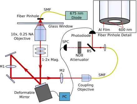
We physically simulate the collection of light from a point-like emitter using a 600-nm pinhole etched through a 200-nm thick aluminum film on the tip of a SMF [Fig. 2, inset]; the result is a highly-divergent source (NA>0.8) of 675-nm light. A 4-mm pane of glass representing, e.g., the vacuum window of a simulated emitter’s setup, separates the pinhole from either a 10X, 0.25-NA microscope objective or a 0.5-NA aspheric lens; these approximately collimate∼500µW (16%) of the collected light and also serve to define the effective numerical aperture of the collection system by clipping the mode emitted from the fiber. Using two-lens imaging we expand the resulting beam to cover the 10.5-mm-diameter surface of our deformable mirror (9.6◦_incidence).

After reflecting from the mirror, the light is collected by a microscope objective and focused onto a single-mode fiber (Thorlabs 460HP). In order to obtain the optimal coupling without the AO mirror, the fiber position is first optimized using a precision piezo-controlled 6-axis stage (APT Nanotrak), though in practice most of the alignment is optimized using only the positional (X/Y/Z) degrees of freedom. The fiber output is then projected through a beamsplitter; the transmitted light is attenuated and sent to a free-space single-photon detector, while light from the reflected port is recorded by a photodiode to monitor the coupling efficiency while the genetic algorithm optimizes single-photon counts.

completely corrected, which limits the maximum coupling achievable in our simulation.

ND8 Attenuator SPC

Photodiode

BS

SMF

Coupling Objective M2

M1

Deformable Mirror 10x, 0.25 NA

Objective

Glass Window Fiber Pinhole

SMF

1-2x Mag.

PC

Fig. 2. Schematic of the experimental setup. Laser light at 675 nm is collected from a pinhole, collimated, and manipulated using a deformable mirror before being contracted (minification lenses M1-2) and focused into a single-mode fiber. The coupling efficiency is monitored using a photodiode, but optimized using a single-photon counter (SPC) after attenuation.

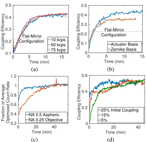
In Fig. 3(a) we show a comparison of the system’s performance for various initial count rates. For lower count rates (10 kcps), the count rate is more significantly affected by shot noise and direct comparison of mirror configuration performance is difficult. Nevertheless, our system is able to optimize collection almost as well as for higher count rates (75 kcps or greater) with a small decrease in optimization speed and an increase in the variability of the final count rate. As shown in Fig. 3(b), use of the actuator basis is better able to correct aberrations in the long term given the higher number of basis elements (all 69 actuators); in contrast, the Zernike basis allows for a faster initial optimization due to a shorter initialization time. The actuator basis was used in all tests (decribed below) for consistency.

Time (min)

0 5 10 15

Coupling Efficiency 0.1 0.2 0.3 0.4 0.5 10 kcps 50 kcps 75 kcps Flat-Mirror Configuration Time (min)

0 5 10 15

Coupling Efficiency 0 0.1 0.2 0.3 0.4 0.5 Actuator Basis Zernike Basis Flat-Mirror Configuration (a) (b) Time (min)

0 20 40

Fraction of Average

Optimized Count Rate 0.2 0.4 0.6 0.8 1 1.2

NA 0.5 Aspheric NA 0.25 Objective

Time (min)

0 20 40

Coupling Efficiency

0 0.2 0.4 0.6

25% Initial Coupling 15%

5%

(c) (d)

Fig. 3. Performance of the algorithm (a) for various initial count rates (in the actuator basis after first optimizing the flat-mirror coupling), showing a robustness against signals affected heavily by shot noise and (b) for optimization in the basis of the first 30 Zernike polynomials or the basis of all 69 mirror actuators. (c) A comparison of AO correction for 1”, 0.5-NA aspheric and 0.25-NA objective collection lenses using the actuator basis, normalized to the average count rate after optimization, in order to emphasize the convergence speed difference. The unnormalized final coupling efficiency with the aspheric lens (<5%) was actually much lower with the objective (50%). (d) Performance for system misalignment where the assumed ‘best’ alignment results in a coupling of 50%. The algorithm is able to correct even severely misaligned systems, with a small cost in optimization time. Each line plots the maximum counts per generation, with the classical coupling given by the monitoring photodiode.

other orders this effect is much less pronounced. This is a limitation of the device itself, and should be reduced significantly for higher-resolution models.

We investigated the effect of the initial system alignment (initial coupling) on the algorithm’s performance. For these tests, the algorithm achieved a 50% coupling efficiency after a manual alignment; the system was then intentionally misaligned varying amounts by tilting the final mirror before the single-mode fiber. Finally, the algorithm-controlled deformable mirror was used to try to compensate for this misalignment. The system was able to correct these issues (Fig. 3d), though the optimization time increased for poorer alignments.

required for these final runs does not necessarily improve the overall optimization efficiency. Monte Carlo simulations of the algorithm indicate that the fastest strategy on average (comparing using a fixed number of children for each iteration, or linearly or exponentially increasing the number of children per iteration) is to fix the number of children at 20 mirror configurations per generation. These simulations also suggest that, for our experimental setup, the algorithm should reach completion after approximately 100 generations (see Appendix A).

4. Application to Quantum Dots

4.1. Stationary Collection

The optimization of light collection is crucial for performing experiments using quantum optics techniques in QD systems [17]. Recent work on spin-photon entanglement using single charged QDs are largely limited by collection efficiency [18–20]. Adaptive optics could have a significant impact on experiments such as entanglement swapping via intermediate entangled photons, and were, in fact, used in recent work using NV centers to perform a loophole-free bell test [21].

We applied our technique to collecting photons from self-assembled InAs quantum dots (QD) grown using molecular beam epitaxy and embedded in a distributed Bragg-reflector (DBR) cavity for enhanced light collection. As shown in Fig. 4(a), the sample is cooled by a liquid-helium optical cryostat; excitation and collection are performed by a high numerical aperture lens (NA=0.68). A Ti:Saph continuous-wave laser is tuned above the∼890-nm band-gap, exciting carriers into the conduction band; these carriers then radiatively recombine at the exciton resonance. The excitation laser (<890 nm) is filtered out by a 925-nm long-pass filter while the QD luminescence (∼950 nm) is sent to a single-grating spectrometer where single dot signatures are seen on a liquid nitrogen-cooled CCD. In order to isolate a single QD for optimization, we use an etalon (10-nm free spectral range, finesse of 100) placed after the long-pass filter. The beam path is sent to a single-mode fiber via the deformable mirror; the fiber output is sent to the spectrometer to verify that only QD luminescence is coupled into the fiber. Finally, a fiber-coupled single-photon avalanche photodiode (SPAD) monitors the single photon counts from the dot and serves as the input for the genetic algorithm software.

Spectrometer/SPC

5K Cryostat QD Sample Deformable Mirror

f = 5 cm Achromats ~10 cm

90/10 BS

890 nm Laser 925 nm Long Pass 30 GHz FSR Etalon

AL

FSW FSW

AL

Time (min)

0 10 20 30 40 50 60

Count Rate (cps)

×104

1.5 2 2.5 3 3.5

Run 1 Run 2 Run 3 Flat-Mirror Configuration

(a) (b)

Fig. 4. Optimizing collection from an InAs quantum dot (QD). (a) Photoluminescence light is collected from the QD and collimated with a focusing asphere (AL, Thorlabs 352330-B) before passing through two fused-silica cryostat windows (FSW, 0.2” and 0.125”, respectively). Two 5-cm focal length achromatic lenses (Thorlabs AC254-050-B-ML) are used for fine adjustment of the beam. The dot light is then filtered with a 925-nm long-pass and a 30-GHz free-spectral-range etalon to remove residual pump light. The filtered QD light is manipulated by the deformable mirror and coupled into a single-mode fiber (SM980) with an aspheric lens (Thorlabs C260TME-B). The light is then sent to a spectrometer to confirm the collection of QD photoluminescence. After tuning the system for a particular QD, the QD emission is sent to a single-photon counter for optimization using our algorithm. (b) Several optimizations of the collection from a single quantum dot, showing up to 50% improvements in coupling. The optimization rate and final count rate were dependent on the overall system alignment and temperature of the dot.

4.2. Simulation of Source Drift

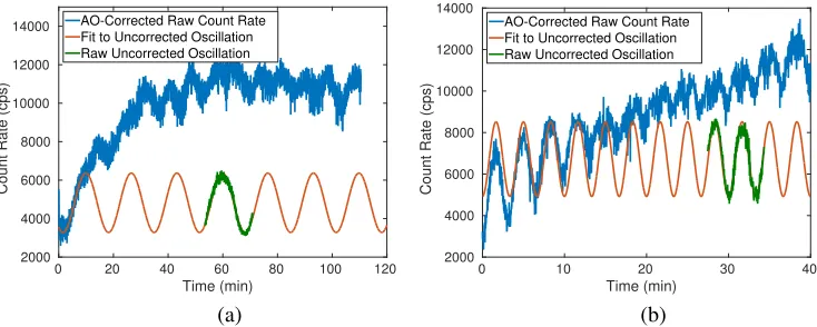
In practice, almost all point emitters that emit into free space are likely to display some amount of drift, e.g., situations where effects such as thermal expansion or ion drift translate the photon source relative to the collection optics. Ideally, the adaptive collection system should compensate for such drifts. Here we evaluate how well our system achieved this. Because our experimental setup did not enable us to realize such a displacement of the actual source in a controllable way, we instead used a piezoelectric translation stage to apply a 3.95-µm peak-to-peak displacement in the horizontal position of the collection fiber with respect to the final coupling lens. The movement of the fiber results in an oscillation in the count rate as seen by the final single-photon detector, just as a lateral shift in the position of the quantum dot emitter would. In this way, we are able to emulate some of the aberrations caused by a slowly moving source.

Time (min)

0 20 40 60 80 100 120

Count Rate (cps)

2000 4000 6000 8000 10000 12000

14000 AO-Corrected Raw Count Rate

Fit to Uncorrected Oscillation Raw Uncorrected Oscillation

Time (min)

0 10 20 30 40

Count Rate (cps)

2000 4000 6000 8000 10000 12000 14000

AO-Corrected Raw Count Rate Fit to Uncorrected Oscillation Raw Uncorrected Oscillation

(a) (b)

Fig. 5. Behavior of the adaptive optic system in the presence of source drift (oscillating count rates of (a) 1000 s period (1 mHz) and (b) 200-s period (5 mHz). Sinusoidal fits to measured oscillations (green data) before correction are shown in red as a guide to the eye. For slow oscillations (>200-s period) the algorithm improved the mean photon count and was able to largely suppress the oscillation amplitude. For faster oscillations, the ability of the algorithm to reduce the oscillation amplitude and improve the mean count rate decreased approximately inversely proportionally to the “drift” rate.

5. Final Notes

In conjunction with a deformable mirror, our algorithm is capable of improving the single-mode fiber coupling of aberrant beams from a variety of sources, including from real-world stationary and drifting light sources. At least 1000 counts per test configuration is desirable for reliable performance; this number may be increased at the cost of overall optimization time (assuming the increase is simply due to longer accumulation times), leading to a reliably higher final coupling efficiency as long as the longer collection time does not approach the timescale of any system drifts. For some single-photon emitter applications, low count rates may increase the overall optimization time to unacceptable levels (e.g., molecules that emit only a finite number of photons before bleaching). One possible solution for some cases is to run the collection system backward, stimulating the emitter with high-intensity light reflected from the deformable mirror and optimizing the counts collected from the subsequent emitter fluorescence over a much larger solid angle, e.g., detected by a camera or large area photomultiplier tube. We have verified that our system performs identically in both the forward (e.g., collection from a pinhole or emitter) and backward (e.g., coupling into a pinhole, or driving an emitter) directions. This is clearly a strategy to be testedin situ, but one that could greatly improve the time for optimizing the coupling between the single-photon emitter and a fiber or other single-mode optical element.

6. Appendix A: Simulations

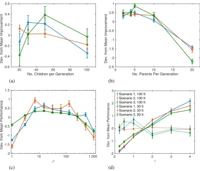
The other parameters influencing our algorithm’s behavior (the number of parentsk, the step rate between generationsγ, the scale of the step rateρ, and the initialization voltageβ) are also tunable by the user. Some of these parameters are situation-dependent; for example, in cases where coupling light from a point emitter is extremely sensitive to very small beam aberrations, using large initial deformations (largeβ) or allowing the children to differ significantly (large ρ) may cause algorithm performance to degrade. However, in some cases we are able to set general guidelines for choosing parameters as a result of numerical simulations of the algorithm. A summary of these results is presented in Fig. 6.

(a)

No. Children per Generation

20 40 60 80 100

Dev. from Mean Improvement

-0.6 -0.4 -0.2 0 0.2 0.4 0.6

(b)

No. Parents Per Generation

0 5 10 15 20

Dev. from Mean Improvement

-2.5 -2 -1.5 -1 -0.5 0 0.5 1

(c)

ρ

1 10 100 1,000

Dev. from Mean Performance

-2 -1.5 -1 -0.5 0 0.5 1 1.5

(d)

0 1 2 3 4

-2 -1 0 1 2 3

Dev. from Mean Performance

Scenario 1, 100 It Scenario 2, 100 It Scenario 3, 100 It Scenario 1, 30 It Scenario 2, 30 It Scenario 3, 30 It

Fig. 6. The results of numerically simulating the genetic algorithm while adjusting various parameters for three aberration scenarios (red, blue, green), adjusted for the final mean performance across the parameter space (i.e.,±1 represents a±100% difference in algorithm performance from the average case). Each plot represents the coupling improvement relative to the starting efficiency using 2000 test configurations (e.g., 100 generations of 20 children). In (a)-(c), the three colored curves represent three different sets of wavefront aberrations to correct. (a) Adjusting the number of child mirror configurations per generationnwhile

keeping the total time constant (total number of test configurations across all generations, where the number of generations is set to 2000/n) suggests that, given a constant 10 parents

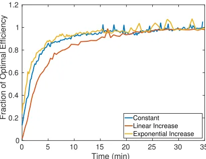
7. Appendix B: Tests of Varying Family Sizes for Pinhole Coupling Optimization Using our pinhole-simulated point source, we experimentally evaluated the algorithm’s perfor-mance as the number of children per generation was varied [Fig. 7]. We compared holding the number constant at 20 children per generation, adding one child every generation (linearly increasing from 20 children), and exponentially increasing the number of children ase0.04m+20, wheremis the generation number. The final optimized value was similar for all cases; however, the optimization speed of the linear case was significantly lower than for the constant or exponential cases. We chose to hold the number of children constant at 20 children per generation for all other tests.

Time (min)

0 5 10 15 20 25 30 35

Fraction of Optimal Efficiency

0 0.2 0.4 0.6 0.8 1 1.2

Constant Linear Increase Exponential Increase

Fig. 7. Experimental algorithm performance as the number of children per generation is varied (holding the generation size at 20 children per generation, increasing linearly from 20 children per generation, and exponentially increasing from 20 children per generation). Each run is normalized to the final optimized value, which was comparable across all cases. The speed of optimization was worst for the linearly-increasing case.

8. Appendix C: Repeated Runs for a Single Quantum Dot

0 1 2 3 4 5 6 7 8 9 10 11 12 13 14 15 16 17 18 19 20 21 22 23 24 25 26 27 28 29 30 Zernike Polynomial (Noll Ordering)

-6 -4 -2 0 2 4 6

Amplitude (arb. units)

10-3

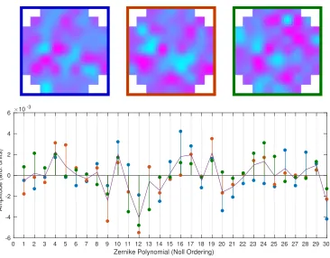
Fig. 8. Zernike amplitudes after optimizing collection from a single quantum dot several times in succession (optimization data presented in main text). The three runs are presented in blue, green, and red, and the solid line displays the average of the three runs. The corresponding final mirror configurations for each run are reproduced above the chart. Actuator voltages of ±0.02 V are magenta and cyan, respectively. The absolute throw per volt is dependent on the overall membrane tension and therefore cannot be estimated directly, but the peak-to-valley displacement is on the order of a few microns or less. There is significant variation in the optimal configuration for each run, which may suggest the presence of higher-order aberrations which are not fully addressable using our finite-resolution mirror.

Funding