Solution of Stochastic Cubic and Quintic Nonlinear Diffusion Equation Using WHEP, Pickard and HPM Methods

(1)

Open Journal of Discrete Mathematics, 2011, 1, 6-21

doi:10.4236/ojdm.2011.11002 Published Online April 2011 (http://www.SciRP.org/journal/ojdm)

Solution of Stochastic Cubic and Quintic Nonlinear

Diffusion Equation Using WHEP, Pickard and

HPM Methods

Magdy A. El-Tawil1_{, Aisha F.Fareed}2

1_{Cairo university, Faculty of Engineering, Engineering, Mathematics Department, Giza, Egypt} 2_{Benha university, Benha Higher Institute of Technology, Basic Science Department, Benha, Egypt}

E-mail:{magdyeltawil, aisha.farid}@yahoo.com

Received March 13, 2011; revised March 23, 2011; accepted April 3, 2011

Abstract

In this paper, the cubic and quintic diffusion equation under stochastic non homogeneity is solved using Wiener- Hermite expansion and perturbation (WHEP) technique, Homotopy perturbation method (HPM) and Pickard approximation technique. The analytic solution of the linear case is obtained using Eigenfunction expansion .The Picard approximation method is used to introduce the first and second order approximate solution for the non linear case. The WHEP technique is also used to obtain approximate solution under dif-ferent orders and difdif-ferent corrections. The Homotopy perturbation method (HPM) is also used to obtain some approximation orders for mean and variance. Using mathematica-5, the methods of solution are illus-trated through figures, comparisons among different methods and some parametric studies.

Keywords:Stochastic Diffusion Equations, WHEP Technique, HPM Method

1. Introduction

The study of random solutions of partial differential equations was initiated by Kampe de Feriet in 1955 [1]. In his valuable survey on the theory of random equations, Bharucha-Reid showed how a stochastic heat equation of Cauchy type can be solved using the stochastic integrals theory[2]. In 1973, Lo Dato V. [3] considered the sto-chastic velocity field and the Navier-Stokes equation and discussed the mathematical problems associated with it. Becus A. Georges [4] introduced a general solution for the heat conduction problem with a random source term and random initial and boundary conditions. Many au-thors investigated the stochastic diffusion equation under different views, see [5-11].

El-Tawil M. used the Wiener-Hermite expansion to-gether with perturbation theory (WHEP technique) to solve a perturbed nonlinear stochastic diffusion equation [12]. The technique has been then developed to be ap-plied on non-perturbed differential equations using the homotopy perturbation method and is called Homotopy WHEP [13,14]. El-Tawil M. and Noha A. El-Molla.[15] solved the quadratic and cubic non-linear stochastic dif-fusion equation using Pickard approximation and

homo-topy WHEP technique [16].

The diffusion equation with cubic and quintic nonlin-ear losses and stochastic non homogeneity are solved using different techniques, mainly the Pickard approxi-mation, the WHEP technique and HPM. The main goal of the paper is to compare among these different tech-niques. Some statistical moments are obtained, mainly the ensemble average, covariance and variance of the solution processes. In Sections 2.1 and 3.1, the Pickard approximation technique is used in solving the cubic and quintic nonlinear diffusion problems respectively. WHEP technique is processed in Sections 2.2 and 3.2, while HPM is used in Sections 2. 3 and 3. 3. Some compari-sons are illustrated in different sections.

2. The Cubic Nonlinear Stochastic Diffusion

Equation

Let us consider the following stochastic nonlinear-diffusion equation with cubic nonlinear losses, ___u3:

 

_{ }

    

  

 

2

2 2

,

;

, 0, 0, , 0, 0, , 0

u x t u

u n x

t x

x t L u t u L t

 

 _ _{ } _{ }

 

(2)

 

and u x,0  x . (1) Where  is a deterministic scale for the nonlinear term. The in homogeneity term n x



;



is space white noise scaled by  .

Three methods are used in the next subsections, mainly the Pickard approximations, the WHEP technique and Homotopy perturbation method.

2.1. Using Pickard Approximation

In this technique, the linear part of the differential op-erator is kept in the left hand side of the equation whereas the rest of the nonlinear terms are moved to the right part. The successive Pickard approximations are processed according to letting the L.H.S. as the n1

approximation for the solution process depending on the approximation in the R.H.S, Following this routine and applying it on to (1), we get the following iterative equations:

th

n n0





 

   

 

2

0 0

2

0 0 0

; 0

0, , ,0 , 0

u u

n x

t x

u x x u t u t L

             (2)





 

2 1 1 2

1 1 1

; , 0

0, , ,0 , 0

n n

n

n n n

u u

n x u n

t x

u x x u t u t L

                    ,  (3) Using Eigen function expansion, the following general solutions are got

 

2

0 0 0

0 0

π

, e sin sin

n L

n n

n

u t x T x I t x

L L     _ _     









nπ (4)

where

 

0

2 π

( )sin d ,

L n

n

F t n x x

L L





_

x (5)

 

2 0 0 e n t _t L n

I t F

 _

0 d

n  

  _ _ 



_

(6) Also,

 

2 1 1 1 0 0 π π

, _n e sin _n sin

m t L

n n n

m m

u t x T x I t

L L       _ _      









x

(7) where

 

1 0 3 0 2 π

( )sin d

2 π

, sin d

n L n L n m

F t n x x x

L L

m

u t x x x

L L     



(8)

 

2

1 π ( ) ( ) 0 e ( n m t _t L n

I  t  Fn_n₁  ) d

 



_

_ (9)

 

1

0

2 π

sin d .

n L n

m

T x

L  L

t x T x

L     _{ }   





. (12) The covariance of u0 is given by

  







   

2 2

2

0 1 0 2 2 ,

0 0 π π 0 0 1 2 4 , , ,

e d e d

π π

sin sin

n m n m

n n

t _t t _t

L L

Cov u t x u t x I

L n m x x L L              _ _  _ _          

 



   (13) where , 0 π π

sin sin d

L n m

n m

I x x

L L



_

x (14) The variance is

 

    2 0 2 π 2 2 , 2

0 0 0 π

0 4

, e

π π

e d sin sin .

n

t _t

L

u n m

n m

n

t _t

L

t x I

L n m d x x L L           _ _      _ _                  

 



(15)

The following results for the first order approxima-tion are obtained:

 

2 0 2 1 π 1 0 π 0 0 π

, e sin

π

e d sin

n t L n n n t _t L n n n

u t x T x

L n F x L         _ _     _ _              



 

(16)

 

1 3 0 0 0

2 π 2 π

sin , sin d

L L

n

n n

F t n x x u t x x

L L L L

 



_



_

_ _ x

(3)

8 M. A. EL-TAWIL ET AL.

 

   

     

0 0 0

3 ₃ ₂

0

0 0

0 0 0

π

, , 3 ( , ) sin

π

3 , sin

π

sin

π

sin

u u n

n

u n m

n m

n m l n m l

n

u t x t x t x I t x

L n

t x I t I t x

L m

x L

n

I t I t I t x

L                       



 

  

π π

sinm xsinl x

L L (18)

 

2 1 0 2 1 π 0 π 0 0 π

, e sin

π

e _n d sin

n t L u n n n t _t L F n n

t x T x

L n _x L           _ _     _ _              



 

(19) where

 



0

 

0

 

0



1

3 2

0

2 _, ₃ _, _{( , )}

π

sin d

n

L

F t u t x u t x u

L n

x x L



 

_

    t x

(20)



 







   

 

1 1 2 1 1 2 1 1 1

1 1 1 2

1 2 0 0 π 2 0 0 1 0 π 1 0 0 2 0 , , , π π sin sin π

e d sin

π

sin

π

e d sin

π sin n m n m n t _t L n n m m m t _t L m m n n n

Cov u t x u t x

n m

EI t I t x x

L L

n

EF x

L

m

EI t x

L

m

EF x

L

n

EI t x

L EI              _ _        _ _                          

 

 



 



 

1 1

 

2

0 0

π π

sin _m sin

n m

t x EI t

L L

 

 





x

(21)

where E denotes the ensemble average operator and

 

2 1 π 0 e n t _t L n

EI t _

_

   EF_n₁  d ₍₂₂₎

   

1 1 2 2 1 2 1 1 π π

1 2 1

0 0

e e d

n m

t t _t _t

L L

n m

EI t I t

EF F   2 d         _ _  _ _     



_{ }

(23)

In which

   

  



  





 



1 1 1 2

2 2

0

3

3 4 3 0 2 4 3 4

2 0 0

3

3 4 4 0 1 3 3 4

2 0 0 2

3 3

3 4 0 1 3 0 2 4 3 4

2 0 0

4 _sin π _sin π _d

4 π π

sin sin , d d

4 _sin π _sin π _, _{d d}

4 _sin π _sin π _, _, _{d d}

n m L L L L L L L EF F

n _x m _{x x}

L L

L

n m

x x En x u x x x

L L

L

n _x m _{x En x u} _x _{x x}

L L

L

n _x m _{x Eu} _{x u} _x _{x x}

L L L     _  _  _ _    





(24) where

   

       

2 0 0

0 0 0

3 0

2 π

0 0

0 0 0 ,

π π

3 e sin sin

π sin π π sin sin n t L n n n n

n m l

En x u t y

n n

T y y En x

L L

n

En x I t I t I t x

L m l x x L L    _{ }                     



  

I t (25) In which

   

  2 0 π 0

2 _sin π t_e n _t _d L n

n

En x I t x

L L



 _  _ _

   



_

(26)

       

     

   

 

0 0 0

2 2 2

1 2 3

0 0 0

π π π

0 0 0

1 2 3 1 2

e e e

d d d

n m l

t t t _t _t _t

L L L

n m l

En x I t I t I t

En x F F F

   3            _ _  _ _  _{ }        

_{  }

 (27) And



 





 





 



   









   



 



   

0 0 0 0 0 0 3 3

0 1 3 0 2 4

3 3 3

1 3 2 4 1 3 2 4

2 2 4 4

0 0

3

2 4 1 3 1 1

0 0

3 3

2 2

1 3 2 4 1 2

0 0

3

, ,

, , 3 , ,

π π

sin sin

3 , ,

π π

sin sin

9 , ,

π sin s n m n m n m n m n m n m

Eu x u x

x x x x

n m

EI I x x

l l

x x EI I

n m

x x

l l

x x EI I

n x l                                        

 





₀

     

₀ ₀

4

2

1 3 1 2 2

0 0 0 0

π

in

3 , n m l

n m l k

m x l

x EI I I

       

   



  



(4)

 





     

 



 



 

     

0

0 0 0

0

0 0 0

2 3 4 4 4

2

2 4 1 1 1

0 0 0 0

2 3 3 3 4

1 3 2 4 1

0 0 0 0

1 2 2

π π π π

sin sin sin sin

3 ,

π π π π

sin sin sin sin 9 , ,

sin

k

n m l

n m l k

k

n

n m l k

m l k

n m l k

I x x x x

l l l l

x EI I I

n m l k

I x x x x

l l l l

x x EI

I I I

                                

  

     

0 0 0

3 3

4 4

1 1 1

0 0 0 0 0 0

2 2 2 3 3

4 4 4

π π

sin

π π

sin sin

π π π

sin sin sin

π π π

sin sin sin

n m l

n m l k v w

k v w

n m x x l l l k x x l l

EI I I

n m l

3

I I I x x

l l l

k v w

x x x

l l l

                  

   

x (28) In which

 

2 0 π 0 π

, e sin

n t L n n n

t x T x

L

     





, (29)

   

0 0

2 2

1 1

1 3 1 4

1 1 π π 2 , 2 0 0

4 _e _e _d

n m n m L L n m EI I I L   _{ } _{ }   

3d 4  

    _ _  _ _ 

   



_{ }

(30)

   

0 0

2 2

2 3 2 4

2 2 π π 2 , 3 2 0 0 4

e e d

n m n m L L n m EI I I L   _{ } _{ }    4 d       _ _  _ _ 



_{ }

(31)

   

0 0

2 2

2 1

1 3 2 4

1 2 π π 2 , 3 2 0 0 4

e e d

n m n m L L n m EI I I L   _{ } _{ }    4 d       _ _  _ _ 



_{ }

(32)

       

 

     

0 0 0 0

2 2 2 2

2 1 1 1 ₁ ₃ ₁ ₄ ₁ ₅ ₂ ₆

0 0 0 0

1 1 1 2

π π π π

0 0 0 0

3 4 5 6 3 4 5 6

e e e e

d d d d ,

n m l k

L L L L

n m l k

EI I I I

EF F F F

    _{ } _{ } _{ } _                     _ _  _ _   _{ }  _ _  

_{   }

 (33)

       

0 0 0 0

2 2 2 2

2 2 2 1

1 3 1 4 2 5 2 6

1 2 2 2

π π π π

0 0 0 0

e e e e

n m l k

L L L L

EI I I I

    _{ } _{ } _{ } _{ }             _ _  _ _  _{ }  _ _          

_{   }

 

   

0 3 0 4 0 5 0 6 d d d d ,3 4 5 6

n m l k

EF  F  F  F      (34)

       

0 0 0 0

2 2 2 2

1 1 2 2

1 3 1 4 2 5 2 6

1 1 2 2

π π π π

0 0 0 0

e e e e

n m l k

L L L L

EI I I I

    _{ } _{ } _{ } _{ }             _ _  _ _  _{ }  _ _          

_{   }

 

   

0 3 0 4 0 5 0 6 3 4 5 6

EFn  Fm  Fl  Fk  d d d d ,    (35)

           

       

   

 

       

0 0 0 0 0 0

2 2 2 2

2 2 2 1 1 1 ₁ ₃ ₁ ₄ ₁ ₅ ₂ ₆

2 2

2 7 2 8

0 0 0 0 0

1 1 1 2 2 2

π π π π

0 0 0 0 0 0

π π

3 4 5 6 7

e e e e

e e

n m l k v w

n m l k

L L L L

v w

L L

n m l k v

EI I I I I I

EF F F F F

      _{ } _{ } _{ } _{ }                        _ _  _ _  _{ }  _ _              _ _  _ _  

_{     }

 

0 8 3 4 5 6 7 8

Fw  d d d d d d ,      (36) where

 

     

0 3 0 4 0 5 0 6

4

1 1 2 2 1

4 0 0 4

1 1 2 2 1

4 0 0 4

1 1 2 2 1

4 0 0

16 _sin π _sin π _sin π _sin π _{d d}

16 π π π π

sin sin sin sin d d

16 π π π π

sin sin sin sin d d .

n m l k

L L L L L L EF 2 2 2

F F F

n _x m _x l _x k _x _{x x}

L L L L

L

n l m k

x x x x x x

L L L L

L

n k m l

x x x x x x

L L L L

L        

 

(37) Using mathematica-5, the previous huge computat w

1 and 2 illustrates the change of the first order m

 

ions ere performed and the following sample results are obtained:

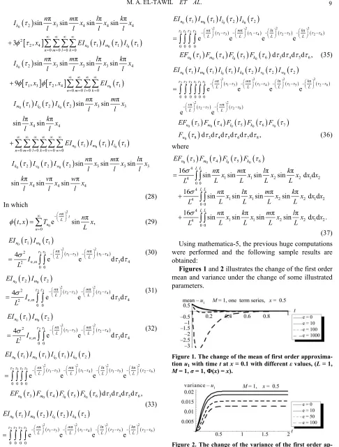
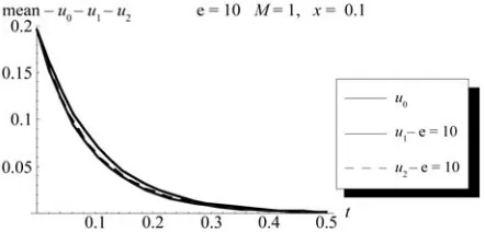
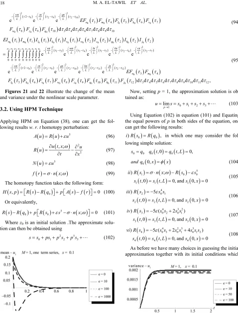
Figures

[image:4.595.62.548.59.700.2]

ean and variance under the change of some illustrated parameters.

Figure 1. The change of the mean of first order approxima-tion u1 with time t at x = 0.1 with different ε values, (L = 1,

M = 1, σ = 1, Φ(x) = x).

Figure 2. The change of the variance of the first order p- a proximation u1 with time t and space variable x at x= 0.5at

[image:4.595.324.531.608.689.2]

(5)

One can notice that the mean diminishes with time for all ε while the variance decreases with the increase of ε.

[image:5.595.64.282.154.244.2]

Following similar computation procedure, the follow-ing results for the second order approximations of the mean is illustrated in Figures 3, 4, 5 and 6.

Figure 3. The change of the mean of second order approxi- mation u2 with time t at x = 0.1with different εvalues, (L

1, M = 1, σ = 1, Φ(x) = x).

[image:5.595.63.284.290.396.2]

=

Figure 4. The change of the mean of zero, first and secon order approximation (u , u , u)with time t at x = 0.1, ε=10, d

0 1 2

(L = 1, M = 1, σ= 1, Φ(x) = x).

Figure 5. The change of the mean of zero, first and seco order approximation (u , u , u0 1 2)with time t at x =0.1, ε=nd50, (L = 1, M = 1, σ = 1, Φ(x)= x).

Figure 6. The change of the mean of zero, first and seco order approximation (u , u , u)with time t at x = 0.1, ε

[25] developed a

nd =

0 1 2

100, (L = 1, M = 1, σ= 1, Φ(x) = x).

2.2. Using WHEP Technique

S th

ince Meecham and his co-workers

eory of turbulence involving a truncated Wiener-Her- mite expansion (WHE) of the velocity field, many au-thors studied problems concerning turbulence [26-27]. A lot of general applications in fluid mechanics was also studied in [28]. Scattering problems attracted the WHE applications through many authors [29]. The nonlinear oscillators were considered as an opened area for the applications of WHE as can be found in [30]. There are a lot of applications in boundary value problems [31] and generally in different mathematical studies [32].

The application of the WHE aims at finding a trun-cated series solution to the solution process of differen-tial equations. The truncated series composes of two major parts; the first is the Gaussian part which consists of the first two terms, while the rest of the series consti-tute the non-Gaussian part. In nonlinear cases, there exist always difficulties of solving the resultant set of deter-ministic integro-differential equations got from the ap-plications of a set of comprehensive averages on the sto-chastic integro-differential equation obtained after the direct application of WHE. Many authors introduced different methods to face these obstacles. Among them, the WHEP technique was introduced in [33] using the perturbation technique to solve perturbed nonlinear problems.

The WHE method utilizes the Wiener-Hermite poly-nomials which are the elements of a complete set of sta-tistically orthogonal random functions [34]. The Wiener- Hermite polynomial  



1, ,2



i

i-1 2

1 2 2

m=1

, , .

, , δ , 2

i

i i i

i i m i

H t t t H t

H t t t t t i



 







  



 

(38)

where

 

_{ }

 

_

_

 

_{ }

 

_

_{ }

_

0

1

2 1 1

1 2 1 2 1 2

3 2 1

1 2 3 1 2 3 1

1

2 3 2 1 3

4 3 1

1 2 3 4 1 2 3 4

2

1 2 3 4 2

1 3 2 4 2

2 3 1 4

1, ,

H , δ , ,

, , H ,

δ δ ,

, , , , ,

H , δ

H , δ ,

H t n t

t t H t H t t t

H

1

H t t t t t H t H t

t t H t t t

H t t t t H t t t H t

t t t t

 

  

    

 

  

[image:5.595.61.288.443.553.2] [image:5.595.62.282.598.683.2]

(6)

In which n(t) is the white noise as noted with the fol-lowing statistical properties

(40) Where δ (-) is the Dirac delta function and. The Wie-ner-Hermite set is a statistically orthogonal set, i.e.

(41) The average of almost all H functions vanishes, par-ticularly,

(42) Due to the completeness of the Wiener-Hermite set, an

 

    

1 2 1 2



0,

δ ,

En t

En t n t t t



  

 i  j ₀ _.

EH H   i j

 i _{0 for} _1.

EH  i

y random function G t

 

; can be expanded as 

 









(0) (1) (1)

1 1 1

(2) (2)

; ;

; , , d d

G t G t G t t H t t

G t t t H t t t t



  

 





1 2 1 2 1 2

 



 



Where the first two terms are the Gaussian pa d

rt of (43)

 

;

G t  .The rest of the terms in the expansion represent the non-Gaussian part of G t

 

; . The average of

 

;

G t  is:

 

_; 0

G EG t G





 



 1

_{ }

 1

_{ }

1 1 1

, ;

; ;

; , d

G G

G

E G t t G

G t t G t t



 2

_

_

 2

_

_

1 2 1 2 1 2

2 G t t t G; , ; ,t t d dt t

     



 

 

  



_



 



_{ }

The variance of G t

 

;

(45)

 i

Var G

s

(46)

The WHEP technique can be applied on lin nonlinear perturbed systems described by ordin partial differential equations. The solution can be modi-fied in the sense that additional parts of the Wiener- Hermite expansion can always be taken into considera-tio ired ord approximations can al-w ending computing tool. It can be even run through a package if it is coded in some sort

of symbolic languages. The technique was successfully applied to several nonlinear stochastic equations, see [20-25].

The first order solution can be obtained when consid-ering only the Gaussian part of the solution process, i.e

 



 



 

_

_

2 1

1 2 2

1 2 1 2

-; ;

d +2 ; , d d

G

t E G t t

G t

G t t t t t

  

 

   

 

 

 

 

 



 

 

t t;1

 2

ear or ary or

 

_

_

 

0 2 0 ₂

0 2

2

0 1

1 1

0 ,

) ,

3 , , ; d ,

x

u t x u

i u t x

t x

u t x u t x x x



  _ _

 _{ } _

 

 



_

_ _ (48)

 

_{ }

 

_{ }

0 _{, 0} _0, 0 _, _{0 and} 0 _0, _,

u t  u t L  u x  x

 

_

_

_

  1

2 ₂

0 1

1

1 2





   

2

1 1

1 1 1

)

, ;

3 , , ;

( ,0; ) 0, ( , ; ) 0 and (0, ; ) 0.

u ii

t

u t x x

u t x u t x x

x

u t x u t L x u x x

 



 _ _

  _ _



  

(49) Applying WHEP technique, the deterministic kernels can be represented in first order approximation as:

(50) (51) Substituting in the previous set of Equations (48) and (49), we get the following four sets of equations:

1 1

0

3 , ; , ; d δ ,

x

u t x x u t x x x x x

   



_

_ _  

 0 (0) (0)

0 1 ,

u u   u

 1 (1) (1)

0 1 .

u u   u

 

_{ }

 

_{ }

 

_{ }

 

_{ }

0 2 0

0 0

2

0 0 0

,

,0 0, , 0 and 0, ,

u t x u

t x

u t u t L u x  x

 



 

  

(52)

0 2 0 ₃

0

1 1

0 2

0 0 0

1 1 1

, ,

,

,0 0, , 0 and

u t x u t x

u t x

t x

u t u t L u

  _ _

 _{ } _

 



0,x 0,

2

0 1

0 0 1

0

3 , , d ,

x

u t x u t x  x

 _ _

 



(53)

 

_

_

1 2 1

0 , ; 1 0 , ; 1

0,

u t x x u t x x

 

 

_

_

1 2

1 1 1

0 1 0 1 0 1

δ

,0; 0, , ; 0 and 0, ;

x x

t x

u t x u t L x u x x



   

 

  

(7)

 

_

_

 

_

_

_

_

1 0.

x 

1 2 1

1 1 1 1

2 2

0 1

0 0 1

2

1 1

0 1 0 1 1

0

1 1 1

1 1 1 1 1

, ; , ;

3 , , ;

3 , ; , ; d

,0; 0, , ; 0 and 0, ;

x

u t x x u t x x

t x

u t x u t x x

u t x x u t x x x

u t x u t L x u x

 



 

 

 _ _ 

 

 _ _

 



(55)

The algorithm of solution is evaluating and first using the separation of variables and t

tion expansion respectively and then computing the other two kernels independently using the Eigenfunction pansion. The final results are:

, , (56)

1

d

eco

(59) The following are some sample r

2.2.1. First Order Approximation and Different Corrections Results

Figures 7 and 8 illustrate the change of the first order mean and variance under different correction l

We can notice the stable results for the different cor-rections.

(0) 0 u

he Eigen

(1) 0 u

ex- 

 0

_{ }

 0

_{ }

0 1

, ,

Eu x t u x t   u x t

 

_

_

 

_

_

 

_

_

 

_

_

2 1

0 1 1

0

1 0

0 1 1 1

0

2 1

2

1 1 1

0

, , ; d

2 , ; , ;

, ; d

x

Var u t x u t x x x

u t x x u t x x x

u t x x x



 

  



 

 _ _



(57)

The result can be made better using the s nd corr tion as the following formula:

 0  0  0

0 1 ,

u u   u (58)

 1  1    1 1 0 1

u u  u₁ . esults.

evels.

Figure 7. Mean comparison between first order with zero, first, second and third corrections at ε = 50 at x = 0.1, (L = 1

= 1, σ = 1, Φ(x)= x).

2.2.2. Sec

, M

ond Order Approximation and Different Corrections Results

igures 9 and 10 illustrate the change of the second or-der mean and variance unor-der different correction levels.

2.2.3. Mean and Variance Comparisons between First and Second Order Approximations with Different Corrections Results

Figures 11 and 12 illustrate in a comparative way, the mean and variance under first and second orders with some correction levels.

[image:7.595.317.532.228.334.2]

F

Figure 8. Variance comparison between first order with first, second and third corrections at x = 0.1 at ε =

, M = 1, σ = 1, Φ(x)= x).

zero, 50,

[image:7.595.61.285.558.685.2]

(L = 1

Figure 9. Mean comparison between second order with zero, first and second corrections at x = 0.1, ε = 50, (L = 1, M = 1,

σ= 1, Φ(x)= x).

Figure 10. Variance comparison between second order with zero, first and second corrections at x = 0.1, ε = 50, (L = 1

M = 1, σ= 1, Φ(x)= x).

[image:7.595.309.540.576.685.2]

(8)

[image:8.595.63.283.77.181.2]

Figure 11. Mean comparison between first order with zero, first, second and third corrections, second order with first and second corrections at x = 0.1 at ε= 30,(L = 1, M = 1, σ= 1, Φ(x)= x).

Figure 12. Variance comparison between first order with zero, first and second corrections at x = 0.1 at ε= 30 (L =

(HPM)

In homotopy Perturbation method (HPM) [18-21], a pa-rameter

1, M = 1, σ= 1, Φ(x)= x).

2.3. Using Homotopy Perturbation Technique

 

0,1

p



is embedded in a homotopy function



,



:



v r p  0,1   which satisfies

, u

B u 0,r

n 



 

 _  

  (62)

ch on nea N,B is a boundary operator, f(r) is a

introdu ,

In which A is a nonlinear differential operator whi can be decomposed into a linear operator R and an

r operator li

known analytic function and Г is the boundary of Φ .the homotopy ces a continuously deformed solution for the case p0 R v

 

L u

 

₀ 0, which is the

he basic idea

original equati f the homotopy method which is to deform continuously a simple le

st

mption of the (HPM) method is that the solution of the original equation can b

po

on .this is t o

prob-m (and easy to solve)into the difficult probleprob-m under udy.

The basic assu

e expanded as a wer series in p as:

2 3

0 1 2 3

v v pv p v p v  (63) Now, setting p = 1, the approxim

tained as:

ation solution is

ob-0 1 2 3

1

lim

p

u v v v v v



      (64) The rate of convergence of the method depends greatly on the initial approximation u0 which is

con-sidered as the main disad tage of M. The idea of imbedded parameter can be utilized to solve nonlinear problems by imbedding this parameter to the problem and then forcing it to be unity in the obtained approxi-mate solution if convergence can be assured .it is a sim-ple

van

Equation (1), we can get the fol-lowingresults w. r. t homotopy perturbation

HP

technique which enables the extension of the appli-cability of the perturbation method from small value ap-plications to general ones.

Applying HPM on

:

 

3

A u R u u (65)

 





22

, ;

u t x u

R u

t x



 

 

  (66)

 

3

N u u (67)

 



0 0 ; 0

R  R z p R z_   n x _ (70) Where z0is an initial solution .The approximate

solu-tion can then be obtained using

2

0 p 1 p

    3

2 p 3

     (71) Now, setting p = 1, the approximation solution is ob-tained as:

0 1 2 3

1

lim

p

u     

 





 

3

1 0 0

) ;

, 0 , 0, and 0

ii R n x R

t t L

    

 

   

 

 

1 1 1 ,x 0

 



2 0 1

2

) 3

, 0

iii R t

  



 



3

4 1

) 6

vi R     

 

0 1 2 0 2

4 4 4

3 ,0

t

    

 





 

t L, 0, and

 

0,x 0 (77) As before we have ma

tion toget

sequent approximation .the choice

0

 is a design problem which can be taken as follows:

 

0

π

, si

π sin d

nt

n n L n

where

 





 

2

π

n t   _t__

1 1

1 0

0 0

0

e d

2

; d

L

n n

L n

j t G

G t n x R x

L

 

   

    



 _    _



3_

(79)

The ensemble averageis

 



_

_  _

covariance is obtained from the following final expression

The

 

_

_

 

_

_





   

2 2

1 2

1 1

1 2

2

1 2

2

1 1 0

π

1 2 0 0

, , ,

4 _sin π _sin π _sin π _sin π _d

d d

L

n m

t t _t _t

Cov u t x u t x

n _x m n m

e L e L

x x

L L L L

L

 _ _



 

   

 

  _   _    

 

 _ _

 

 

 

 





(81) The variance can then be obtained from equation (81) by setting x1 = x2 = x.

Any higher order approximations can be obtai

similar way. The following sample results using the same data in the cubic case.

Computing the consequent errors by using the following expression

x x

   

 

 

ned in a

i Er

1, 1, 2,3, 4

i i i i

Er  mean mean i (82)

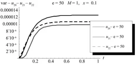
We obtain the following results. Figures 13 illustrates different mean approximations using homotopy method (HPM) with computing their corresponding decreasing errors in Figure 14.

[image:9.595.306.542.406.544.2]

Figures 15 illustrates different variance approxima-tions using homotopy method (HPM) with computing their corresponding decreasing errors in Figure 16.

[image:9.595.58.286.451.690.2]

Figure 13. The mean at different homotopy orders, cubic case.

(10)

[image:10.595.56.281.78.197.2]

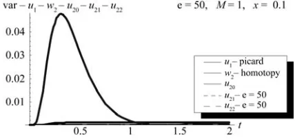
Figure 15. The variance (-1: first and-2: second) at different

[image:10.595.319.531.88.195.2]

ε, HPM, cubic nonlinear case.

Figure 16. The error difference of first and second error at different ε, cubic case.

2.4. Mean and Variance Comparisons of the Solution of Stochastic Cubic Nonlinear Diffusion Problem Using WHEP, Pickard and HPM Methods with Different Orders and Corrections

Figures 17, 18, 19 and 20 illustrate some useful com-parisons among the three used methods in this paper.

3. The Quintic Nonlinear Stochastic

et us consider the following stochastic nonlinear-diffusion equation

Diffusion Equation

L





_

_

  

    

 

2

5 2 , ;

; ;

, 0, 0, , ,0 0, ,

and 0, .

u t x u

u n x

t x

t x L u t u t L

u x x



  



 _ _{ } _{ }

 

    



0 (83)

Where εis a deterministic scale for the nonlinear term. Two methods are used in the next subsections, mainly the Pickard approximations and the HPM technique.

rd Approximation

he following results for the first order approximation 3.1. Using the Picka

T

are obtained

F

Higomotopy first order and WHEP first order with zero, first, ure 17. Mean comparison between Picard first order, second and third corrections at x = 0.1, ε= 50, (L = 1, M = 1,

[image:10.595.318.532.260.360.2]

σ = 1, Φ(x)= x).

Figure 18. Variance comparison between Picard first order, omotopy second order and WHEP first order with zero, H

first, second and third corrections at x = 0.1, ε= 30, (L = 1, M = 1, σ= 1, Φ(x) = x).

Figure 19. Mean comparison between Picard second order , Homotopy fourth order and WHEP second order with zero, first, second and third correctionsat x = 0.5 , ε= 50,(L = 1, M = 1, σ= 1, Φ(x)= x).

Figure 20. Variance comparison between Picard first order, Homotopy second order and WHEP second order with zero, first and second corrections at x = 0.1, ε= 50, (L = 1, M = 1,

[image:10.595.324.526.423.513.2] [image:10.595.318.532.576.678.2]