Generating Non Projective Word Order in Statistical Linearization

Generating Non-Projective Word Order in Statistical Linearization

Bernd Bohnet Anders Bj¨orkelund Jonas Kuhn Wolfgang Seeker Sina Zarrieß Institut f¨ur Maschinelle Sprachverarbeitung

University of Stuttgart

{bohnetbd,anders,jonas,seeker,zarriesa}@ims.uni-stuttgart.de

Abstract

We propose a technique to generate non-projective word orders in an efficient statisti-cal linearization system. Our approach pre-dictsliftingsof edges in an unordered syntac-tic tree by means of a classifier, and uses a projective algorithm for tree linearization. We obtain statistically significant improvements on six typologically different languages: En-glish, German, Dutch, Danish, Hungarian, and Czech.

1 Introduction

There is a growing interest in language-independent data-driven approaches to natural language genera-tion (NLG). An important subtask of NLG is sur-face realization, which was recently addressed in the 2011 Shared Task on Surface Realisation (Belz et al., 2011). Here, the input is a linguistic representa-tion, such as a syntactic dependency tree lacking all precedence information, and the task is to determine a natural, coherent linearization of the words.

The standard data-driven approach is to traverse the dependency tree deciding locally at each node on the relative order of the head and its children. The shared task results have proven this approach to be both effective and efficient when applied to English.

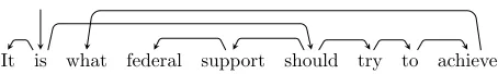
It is what federal support should try to achieve

SBJ ROOT

OBJ

NMOD SBJ PRD

VC OPRD IM

Figure 1: A non-projective example from the CoNLL 2009 Shared Task data set for parsing (Hajiˇc et al., 2009).

However, the approach can only generate pro-jective word orders (which can be drawn with-out any crossing edges). Figure 1 shows a non-projective word order: the edge connecting the ex-tracted wh-pronoun with its head crosses another edge. Once what has been ordered relative to

achieve, there are no ways of inserting intervening material. In this case, only ungrammatical lineariza-tions can be produced from the unordered input tree:

(1) a. *It is federal support should try to what achieve b. *It is federal support should try to achieve what c. *It is try to achieve what federal support should

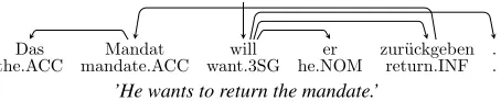
Although rather infrequent in English, non-projective word orders are quite common in lan-guages with a less restrictive word order. In these languages, it is often possible to find a grammati-cally correctprojectivelinearization for a given in-put tree, but discourse coherence, information struc-ture, and stylistic factors will often make speak-ers prefer some non-projective word order.1 Figure 2 shows an object fronting example from German where the edge between the subject and the finite verb crosses the edge between the object and the full verb. Various other constructions, such as extraposi-tion of (relative) clauses or scrambling, can lead to non-projectivity. In languages where word order is driven to an even larger degree by information struc-ture, such as Czech and Hungarian, non-projectivity can likewise result from various ordering decisions. These phenomena have been studied extensively in

1

A categorization of non-projective edges in the Prague Dependency Treebank (B¨ohmov´a et al., 2000) is presented in Hajiˇcov´a et al. (2004).

the linguistic literature, and for certain languages, work on rule-based generation has addressed certain aspects of the problem.

Das Mandat will er zur¨uckgeben .

the.ACC mandate.ACC want.3SG he.NOM return.INF .

NK

OA# –

SB OC –

’He wants to return the mandate.’

Figure 2: German object fronting with complex verb in-troducing a non-projective edge.

In this paper, we aim for a general data-driven ap-proach that can deal with various causes for non-projectivity and will work for typologically dif-ferent languages. Our technique is inspired by work in data-driven multilingual parsing, where non-projectivity has received considerable attention. In pseudo-projective parsing (Kahane et al., 1998; Nivre and Nilsson, 2005), the parsing algorithm is restricted to projective structures, but the issue is side-stepped by converting non-projective structures to projective ones prior to training and application, and then restoring the original structure afterwards.

Similarly, we split the linearization task in two stages: initially, the input tree is modified by lifting certain edges in such a way that new orderings be-come possible even under a projectivity constraint; the second stage is the original, projective lineariza-tion step. In parsing, projectivizalineariza-tion is a determin-istic process that lifts edges based on the linear or-der of a sentence. Since the linear oror-der is exactly what we aim to produce, this deterministic conver-sion cannot be applied before linearization. There-fore, we use a statistical classifier as our initial lift-ing component. This classifier has to be trained on suitable data, and it is an empirical question whether the projective linearizer can take advantage of this preceding lifting step.

We present experiments on six languages with varying degrees of non-projective structures: En-glish, German, Dutch, Danish, Czech and Hungar-ian, which exhibit substantially different word order properties. Our approach achieves significant im-provements on all six languages. On German, we also report results of a pilot human evaluation.

2 Related Work

An important concept for tree linearization areword order domains(Reape, 1989). The domains are bags of words (constituents) that are not allowed to be dis-continuous. A straightforward method to obtain the word order domains from dependency trees and to order the words in the tree is to use each word and its children as domain and then to order the domains and contained words recursively. As outlined in the introduction, the direct mapping of syntactic trees to domains does not provide the possibility to obtain all possible correct word orders.

Linearization systems can be roughly distin-guished as either rule-based or statistical systems. In the 2011 Shared Task on Surface Realisation (Belz et al., 2011), the top performing systems were all statistical dependency realizers (Bohnet et al., 2011; Guo et al., 2011; Stent, 2011).

Grammar-based approaches map dependency structures or phrase structures to a tree that repre-sents the linear precedence. These approaches are mostly able to generate non-projective word orders. Early work was nearly exclusively applied to phrase structure grammars (e.g. (Kathol and Pollard, 1995; Rambow and Joshi, 1994; Langkilde and Knight, 1998)). Concerning dependency-based frameworks, Br¨oker (1998) used the concept of word order do-mains to separate surface realization from linear precedence trees. Similarly, Duchier and Debus-mann (2001) differentiate Immediate Dominance trees (ID-trees) from Linear Precedence trees (LP-trees). Gerdes and Kahane (2001) apply a hierarchi-cal topologihierarchi-cal model for generating German word order. Bohnet (2004) employs graph grammars to map between dependency trees and linear prece-dence trees represented as hierarchical graphs. In the frameworks of HPSG, LFG, and CCG, a grammar-based generator produces word order candidates that might be non-projective, and a ranker is used to se-lect the best surface realization (Cahill et al., 2007; White and Rajkumar, 2009).

(Filip-pova and Strube, 2007; Bohnet et al., 2010) or top-down (Guo et al., 2011; Bohnet et al., 2011). These linearizers are mostly applied to English and do not deal with non-projective word orders. An excep-tion is Filippova and Strube (2007), who contribute a study on the treatment of preverbal and postver-bal constituents for German focusing on constituent order at the sentence level. The work most similar to ours is that of Gamon et al. (2002). They use machine-learning techniques to lift edges in a pre-processing step to a surface realizer. Their objec-tive is the same as ours: by lifting, they avoid cross-ing edges. However, contrary to our work, they use phrase-structure syntax and focus on a limited num-ber of cases of crossing branches in German only.

3 Lifting Dependency Edges

In this section, we describe the first of the two stages in our approach, namely the classifier that lifts edges in dependency trees. The classifier we aim to train is meant to predict liftings on a given unordered de-pendency tree, yielding a tree that, with a perfect lin-earization, would not have any non-projective edges.

3.1 Preliminaries

The dependency trees we consider are of the form displayed in Figure 1. More precisely, all words (or nodes) form a rooted tree, where every node has ex-actly one parent (orhead). Edges point from head to dependent, denoted in the text byh→d, whereh is the head anddthe dependent. All nodes directly or transitively depend on an artificial root node (de-picted in Figure 1 as the incoming edge tois).

We say that a node adominatesa node difais an ancestor ofd. An edgeh → dis projectiveiff hdominates all nodes in the linear span between h

and d. Otherwise it is non-projective. Moreover,

a dependency tree is projective iff all its edges are projective. Otherwise it is non-projective.

Aliftingof an edgeh→d(or simply of the node

d) is an operation that replacesh → dwithg → d,

given that there exists an edgeg→hin the tree, and undefined otherwise (i.e. the dependent d is reat-tached to the head of its head).2 _{When the lifting}

2

The undefined case occurs only when ddepends on the root, and hence cannot be lifted further; but these edges are by definition projective, since the root dominates the entire tree.

operation is appliednsuccessive times to the same node, we say the node was liftednsteps.

3.2 Training

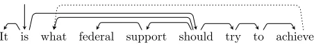
During training we make use of the projectivization algorithm described by Nivre and Nilsson (2005). It works by iteratively lifting the shortest non-projective edges until the tree is non-projective. Here, shortest edge refers to the edge spanning over the fewest number of words. Since finding the shortest edge relies on the linear order, instead of lifting the shortest edge, we lift non-projective edges ordered by depth in the tree, starting with the deepest nested edge. A lifted version of the tree from Figure 1 is shown in Figure 3. The edge ofwhathas been lifted three steps (the original edge is dotted), and the tree is no longer non-projective.

It is what federal support should try to achieve

SBJ ROOT

OBJ

OBJ NMOD SBJ PRD

VC OPRD IM

Figure 3: The sentence from Figure 1, where whathas been assigned a new head (solid line). The original edge is dotted.

We model the edge lifting problem as a multi-class multi-classification problem and consider nodes one at a time and ask the question “How far should this edge be lifted?”, where classes correspond to lifting 0,1,2, ..., n steps. To create training instances we use the projectivization algorithm mentioned above. We traverse the nodes of the tree sorted by depth. For multiple nodes at the same depth, ties are broken by linear order, i.e. for multiple nodes at the same depth, the leftmost is visited first. When a node is visited, we create a training instance out of it. Its class is determined by the number of steps it would be lifted by the projectivization algorithm given the linear order (in most cases the class corresponds to no lifting, since most edges are projective). As we traverse the nodes, we also execute the liftings (if any) and update the tree on the fly.

The training instances derived are used to train a logistic regression classifier using the LIBLINEAR

Atomic features

∀x∈ {w, wp, wgp, wch, ws, wun} morph(x), label(x), lemma(x), PoS(x)

∀x∈ {wgc,wne,wco} label(x), lemma(x), PoS(x)

Complex features

∀x∈ {w, wp, wgp} lemma(x)+PoS(x), label(x)+PoS(x), label(x)+lemma(x)

∀x∈ {wch, ws, wun}, y=w lemma(x)+lemma(y), PoS(y)+lemma(x), PoS(y)+lemma(x)

∀x∈ {w, wp, wgp}, y=HEAD(x) lemma(x)+lemma(y), lemma(x)+PoS(y), PoS(x)+lemma(y)

∀x∈ {w, wp, wgp}, y=HEAD(x), z=HEAD(y) PoS(x)+PoS(y)+PoS(z), label(x)+label(y)+label(z)

∀x∈ {wch, ws, wun}, y=HEAD(x), z=HEAD(y) PoS(x)+PoS(y)+PoS(z), label(x)+label(y)+label(z)

Non-binary features

∀x∈ {w, wp, wgp} SUBTREESIZE(x), RELSUBTREESIZE(x)

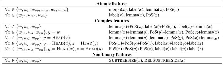
Table 1: Features used for lifting. wrefers to the word (dependent) in question. And with respect tow,wp is the

parent; wgpis the grandparent; wch are children;wsare siblings;wun are uncles (i.e. children of the grandparent,

excluding the parent);wgcare grandchildren;wneare nephews (i.e. grandchildren of the parent that are not children

ofw);wcoare cousins (i.e. grandchildren of the grandparent that are notwor siblings ofw). The non-binary feature

functions refer to: SUBTREESIZE– the absolute number of nodes belowx, RELSUBTREESIZE– the relative size of the subtree rooted atxwith respect to the whole tree.

involve the lemma, dependency edge label, part-of-speech tag, and morphological features of the node in question, and of several neighboring nodes in the dependency tree. We also have a few non-binary fea-tures that encode the size of the subtree headed by the node and its ancestors.

We ran preliminary experiments to determine the optimal architecture. First, other ways of modeling the liftings are conceivable. To find new reattach-ment points, Gamon et al. (2002) propose two other ways, both using a binary classifier: applying the classifier to each node xalong the path to the root asking “Shoulddbe reattached tox?”; or lifting one step at a time and applying the classifier iteratively until it says stop. They found that the latter outper-formed the former. We tried this method, but found that it was inferior to the multi-class model and more frequently over- or underlifted.

Second, to avoid data sparseness for infrequent lifting distances, we introduce a maximum number of liftings. We found that a maximum of 3 gave the best performance. In the pseudocode below, we re-fer to this number asmaxsteps.3 This means that we are able to predict the correct lifting for most (but not all) of the non-projective edges in our data sets (cf. Table 3).

Third, as Nivre and Nilsson (2005) do for

pars-3_{During training, nodes that are lifted further thanmaxsteps} are assigned to the class corresponding tomaxsteps. This ap-proach worked better than ignoring the training instance or treating it as a non-lifting (i.e. a lifting of 0 steps).

ing, we experimented with marking edges that were lifted by indicating this on the edge labels. In the case of parsing, this step is necessary in order to re-verse the liftings in the parser output. In our case, it could potentially be beneficial for both the lifting classifier, and for the linearizer. However, we found that marking liftings at best gave similar results as not marking, so we kept the original labels without marking.

3.3 Decoding

In the decoding stage, an unordered tree is given and the goal is to lift edges that would be non-projective with respect to the gold linear order. Similarly to how training instances are derived, the decoding al-gorithm traverses the tree bottom-up and visits every node once. Ties between nodes at the same depth are broken in an arbitrary but deterministic way. When a node is visited, the classifier is applied and the cor-responding lifting is executed. Pseudocode is given in Algorithm 1.4

Different orderings of nodes at the same depth can lead to different lifts. The reason is that lift-ings are applied immediately and this influences the features when subsequent nodes are considered. For instance, consider two sibling nodes ni and nj. If

ni is visited before nj, and ni is lifted, this means

4_{The M}

that at the time we visitnj,niis no longer a sibling

ofnj, but rather an uncle. An obvious extension of

the decoding algorithm presented above is to apply beam search. This allows us to considernj both in

the context wherenihas been lifted and when it has

not been lifted.

1 N←NODES(T)

2 SORT-BY-DEPTH-BREAK-TIES-ARBITRARILY(N, T)

3 foreachnode∈Ndo

4 feats←EXTRACT-FEATURES(node, T)

5 steps←CLASSIFY(f eats)

6 steps←MIN(steps,ROOT-DIST(node))

7 LIFT(node, T, steps)

8 returnT

Algorithm 1: Greedy decoding for lifting.

Pseudocode for the beam search decoder is given in Algorithm 2. The algorithm keeps an agenda of trees to explore as each node is visited. For every node, it clones the current tree and applies every pos-sible lifting. Every tree also has an associated score, which is the sum of the scores of each lifting so far. The score of a lifting is defined to be the log proba-bility returned from the logistic classifier. After ex-ploring all trees in the agenda, the k-best new trees from the beam are extracted and put back into the agenda. When all nodes have been visited, the best tree in the agenda is returned. For the experiments the beam size (kin Algorithm 2) was set to 20.

1 N←NODES(T)

2 SORT-BY-DEPTH-BREAK-TIES-ARBITRARILY(N, T)

3 Tscore←0

4 Agenda← {T} 5 foreachnode∈Ndo

6 Beam← ∅

7 foreachtree∈Agendado

8 feats←EXTRACT-FEATURES(node, tree)

9 m←MIN(maxsteps,ROOT-DIST(node))

10 foreach s∈0 .. maxstepsdo 11 t←CLONE(tree)

12 score←GET-LIFT-SCORE(f eats, s)

13 tscore=tscore+score

14 LIFT(node, t, s)

15 Beam←Beam∪ {t}

16 Agenda←EXTRACTKBEST(Beam, k)

17 returnEXTRACTKBEST(Agenda,1)

Algorithm 2: Beam decoding for lifting.

While beam search allows us to explore the search space somewhat more thoroughly, a large number of

possibilities remain unaccounted for. Again, con-sider the sibling nodesniandnj whenni is visited

beforenj. The beam allows us to considernj both

when ni is lifted and when it is not. However, the

situation wherenj is visitedbefore ni is still never

considered. Ideally, all permutations of nodes at the same depth should be explored before moving on. Unfortunately this leads to a combinatorial explo-sion of permutations, and exhaustive search is not tractable. As an approximation, we create two or-derings and run the beam search twice. The dif-ference between the orderings is that in the second one all ties are reversed. As thisbibeamconsistently improved over the beam in Algorithm 2, we only present these results in Section 5 (there denoted sim-plyBeam).

4 Linearization

A linearizer searches for the optimal word order given an unordered dependency tree, where the op-timal word order is defined as the single reference order of the dependency tree in the gold standard. We employ a statistical linearizer that is trained on a corpus of pairs consisting of unordered dependency trees and their corresponding sentences. The lin-earization method consists of the following steps:

Creating word order domains. In the first step, we build the word order domains dh for all nodes

h ∈y of a dependency treey. A domain is defined as a node and all of its direct dependents. For ex-ample, the tree shown in Figure 3 has the following domains: {it, be, should},{what, support, should, try},

{federal, support},{try, to},{to, achieve}

If an edge was lifted before the linearization, the lifted node will end up in the word order domain of its new head rather than in the domain of its original head. This way, the linearizer can deduce word or-ders that would result in non-projective structures in the non-lifted tree.

1 //T is the dependency tree with lifted nodes 2 beam-size←1000

3 for h∈Tdo

4 domainh←GET-DOMAIN(T,h)

5 // initialize the beam with a empty word list 6 Agendah←()

7 foreachw∈domainhdo

8 // beam for extending word order lists

9 Beam←()

10 foreach l∈Agendahdo

11 // clone listland append the word w

12 ifw6∈lthen

13 l0←APPEND(l,m)

14 Beam←Beam⊕l0

15 score[l0]←COMPUTE-SCORE(l0) 16 if |Beam|>beam-sizethen

17 SORT-LISTS-DESCENDING-TO

-SCORE(Beam,score)

18 Agendah←SUBLIST(0,beam-size,Beam)

19 else

20 Agendah←Beam

21 foreach l∈Beamdo

22 SCOREg[l]←SCORE[l]+

GLOBAL-SCORE(l)

23 Agendah←Beam

24 returnBeam

Algorithm 3: Dependency Tree Linearization.

The linearization algorithm initializes the word order beam (agendah) with an empty order () (line

6). It then iterates over the words of a domain (lines 7-20). In the first iteration, the algorithm clones and extends the empty word order list () by each word of the sentence (line 12-15). If the beam (beam) exceeds a certain size (beam-size), it is sorted by score and pruned to maximum beam size ( beam-size) (lines 16-20). The following example illus-trates the extensions of the beam for the top domain shown in Figure 3.

Iter. agendabe

0: ()

1: ((it) (be) (should))

2: ((it be) (it should) (be it) (be should) ...)

The beam enables us to apply features that encode information about the first tokens and the last token, which are important for generating, e.g. the word order of questions, i. e. if the last token is a question mark then the sentence should probably be a ques-tion (cf. feature set shown in Table 2). Furthermore, the beam enables us to generate alternative lineariza-tions. For this, the algorithm iterates over the

alter-native word orders of the domains in order to as-semble different word orders on the sentence level.5 Finally, when traversing the tree bottom-up, the al-gorithm has to use the different orders of the already ordered subtrees as context, which also requires a search over alternative word orders of the domains.

Training of the Linearizer. We use MIRA

(Crammer et al., 2006) for the training of the lin-earizer. The classifier provides a score that we use to rank the alternative word orders. Algorithm 3 calls two functions to compute the score: compute-score

(line 15) for features based on pairs of words and tri-grams andcompute-global-scorefor features based on word patterns of a domain. Table 2 shows the feature set for the two functions. In the case that the linearization of a word order domain is incorrect the algorithm updates its weight vectorw. The follow-ing equation shows the update function of the weight vector:

w=w+τh(φ(dh, T, xg)−φ(dh, T, xp))

We update the weight vectorwby adding the dif-ference of the feature vector representation of the correct linearization xg and the wrongly predicted

linearizationxp, multiplied byτ. τ is the

passive-aggressive update factor as defined below. The suf-feredlosshisφ(dh, T, xp)−φ(dh, T, xg).

τ = lossh

||φ(dh,T ,xg)−φ(dh,T ,xp)||2

Creating the word order of a sentence. The lin-earizer traverses the tree either top-down or bottom-up and assembles the results in the surface order. The bottom-up linearization algorithm can take into account features drawn from the already ordered subtrees while the top-down algorithm can employ as context only the unordered nodes. However, the bottom-up algorithm additionally has to carry out a search over the alternative linearization of the sub-domains, as different orders of the subdomain pro-vide different context features. This leads to a higher linearization time. We implemented both, but could only find a rather small accuracy difference. In the following, we therefore present results only for the top-down method.

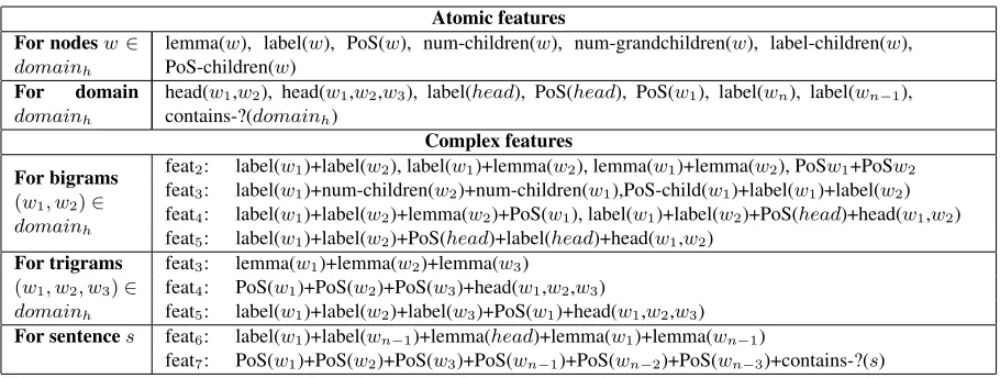
Atomic features For nodesw∈

domainh

lemma(w), label(w), PoS(w), num-children(w), num-grandchildren(w), label-children(w), PoS-children(w)

For domain

domainh

head(w1,w2), head(w1,w2,w3), label(head), PoS(head), PoS(w1), label(wn), label(wn−1),

contains-?(domainh)

Complex features

For bigrams

(w1, w2)∈

domainh

feat2: label(w1)+label(w2), label(w1)+lemma(w2), lemma(w1)+lemma(w2), PoSw1+PoSw2

feat3: label(w1)+num-children(w2)+num-children(w1),PoS-child(w1)+label(w1)+label(w2)

feat4: label(w1)+label(w2)+lemma(w2)+PoS(w1), label(w1)+label(w2)+PoS(head)+head(w1,w2)

feat5: label(w1)+label(w2)+PoS(head)+label(head)+head(w1,w2) For trigrams

(w1, w2, w3)∈

domainh

feat3: lemma(w1)+lemma(w2)+lemma(w3)

feat4: PoS(w1)+PoS(w2)+PoS(w3)+head(w1,w2,w3)

feat5: label(w1)+label(w2)+label(w3)+PoS(w1)+head(w1,w2,w3) For sentences feat6: label(w1)+label(wn−1)+lemma(head)+lemma(w1)+lemma(wn−1)

feat7: PoS(w1)+PoS(w2)+PoS(w3)+PoS(wn−1)+PoS(wn−2)+PoS(wn−3)+contains-?(s)

Table 2: Exemplified features used for scoring linearizations of a word order domain (see Algorithm 3). Atomic features which represent properties of a node or a domain are conjoined into feature vectors of different lengths. Linearizations are scored based on bigrams, trigrams, and global sentence-level features.

5 Experiments

We conduct experiments on six European languages with varying degrees of word order restrictions: While English word order is very restrictive, Czech and Hungarian exhibit few word order constraints. Danish, Dutch, and German (so-called V2, i. e. verb-second, languages) show a relatively free word order that is however more restrictive than in Hun-garian or Czech. The English and the Czech data are from the CoNLL 2009 Shared Task data sets (Hajiˇc et al., 2009). The Danish and the Dutch data are from the CoNLL 2006 Shared Task data sets (Buchholz and Marsi, 2006). For Hungarian, we use the Hungarian Dependency Treebank (Vincze et al., 2010), and for German, we use a dependency con-version by Seeker and Kuhn (2012).

# sent’s np sent’s np edges np≤3 lifts English 39,279 7.63 % 0.39% 98.39%

German 36,000 28.71% 2.34% 94.98%

Dutch 13,349 36.44% 5.42% 99.80%

Danish 5,190 15.62 % 1.00% 96.72%

Hungarian 61,034 15.81% 1.45% 99.82%

Czech 38,727 22.42% 1.86% 99.84%

Table 3: Size of training sets, percentage of non-projective (np) sentences and edges, percentage of np edges covered by 3 lifting steps.

Table 3 shows the sizes of the training corpora and the percentage of non-projective sentences and edges in the data. Note that the data sets for

Dan-ish and Dutch are quite small. EnglDan-ish has the least percentage of non-projective edges. Czech, Ger-man, and Dutch show the highest percentage of non-projective edges. The last column shows the per-centage of non-projective edges that can be made projective by at most 3 lifting steps.

5.1 Setup

In our two-stage approach, we first train the lifting classifier. The results for this classifier are reported in Section 5.2.

Second, we train the linearizer on the output of the lifting classifier. To assess the impact of the lifting technique on linearization, we built four sys-tems on each language: (a) a linearizer trained on the original, non-lifted dependency structures ( No-lift), two trained on the automatically lifted edges (comparing (b) the beam and (c) greedy decoding), (d) one trained on the oracle, i. e. gold-lifted struc-tures, which gives us an upper bound for the lifting technique. The linearization results are reported in Section 5.3.

5.2 Lifting results

To evaluate the performance of the lifting classifier, we present precision, recall, and F-measure results for each language. We also compute the percentage of sentences that were handled perfectly by the lift-ing classifier. Precision and recall are defined the usual way in terms of true positives, false positives, and false negatives, where true positives are edges that should be lifted and were lifted correctly; false positives are edges that should not be lifted but were

andedges that should be lifted and were lifted, but were reattached in the wrong place; false negatives are edges that should be lifted but were not.

The performance of both the greedy decoder and the bibeam decoder are shown in Table 4. The scores are taken on the cross-validation on the training set, as this provides more reliable figures. The scores are micro-averaged, i.e. all folds are concatenated and compared to the entire training set.

Although the major evaluation of the lifting is given by the performance of the linearizer, Table 4 gives us some clues about the lifting. We see that precision is generally much higher than recall. We believe this is related to the fact that some phenom-ena encoded by non-projective edges are more sys-tematic and thus easier to learn than others (e. g. wh-extraction vs. relative clause extraposition). We also find that beam search consistently yields modest in-creases in performance.

Greedy Beam

P R F1 Perfect P R F1 Perfect Eng 77.31 50.45 61.05 95.76 78.85 50.63 61.66 95.83 Ger 72.33 63.59 67.68 81.91 72.05 64.41 68.02 81.97 Dut 76.66 74.89 75.77 79.28 78.07 76.49 77.27 80.34 Dan 85.90 58.55 69.64 92.76 85.90 58.55 69.64 92.74 Hun 72.60 61.61 66.66 88.46 73.06 64.77 68.67 88.73 Cze 77.79 55.00 64.44 86.28 77.31 55.68 64.74 86.33

Table 4: Precision, recall, F-measure and perfect projec-tivization results for the lifting classifier.

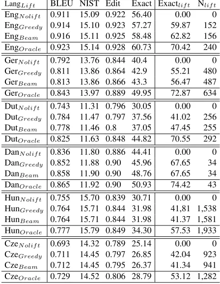
5.3 Linearization Results and Discussion

We evaluate the linearizer with standard metrics: n-gram overlap measures (BLEU, NIST), edit distance (Edit), and the proportion of exactly linearized sen-tences (Exact). As a means to assess the impact of lifting more precisely, we propose the word-based measure Exactlif t which only looks at the words

with an incoming lifted edge. The Exactlif t score

then corresponds to the percentage of these words that has been realized in the exact same position as in the original sentence.

LangLif t BLEU NIST Edit Exact Exactlif t Nlif t

EngN olif t 0.911 15.09 0.922 56.40 0.00 0

EngGreedy 0.914 15.10 0.923 57.27 59.87 152

EngBeam 0.916 15.11 0.925 58.48 62.82 156

EngOracle 0.923 15.14 0.928 60.73 70.42 240

GerN olif t 0.792 13.76 0.844 40.4 0.00 0

GerGreedy 0.811 13.86 0.864 42.9 55.21 480

GerBeam 0.813 13.86 0.866 43.3 56.47 487

GerOracle 0.843 13.97 0.889 49.95 72.87 634

DutN olif t 0.743 11.31 0.796 30.05 0.00 0

DutGreedy 0.784 11.47 0.797 37.56 41.02 256

DutBeam 0.778 11.46 0.8 37.05 47.45 255

DutOracle 0.825 11.63 0.848 44.82 70.55 292

DanN olif t 0.836 11.80 0.886 44.41 0.00 0

DanGreedy 0.852 11.88 0.90 45.96 67.65 34

DanBeam 0.858 11.90 0.90 48.76 67.65 34

DanOracle 0.865 11.92 0.90 50.93 74.42 43

HunN olif t 0.755 15.70 0.839 30.71 0.00 0

HunGreedy 0.764 15.71 0.844 31.98 41,81 1,538

HunBeam 0.764 15.71 0.844 31.98 41.37 1,581

HunOracle 0.777 15.79 0.849 34.30 57.53 1,933

CzeN olif t 0.693 14.32 0.789 25.14 0.00 0

CzeGreedy 0.711 14.45 0.797 26.85 42.04 923

CzeBeam 0.712 14.45 0.795 26.37 41.34 941

CzeOracle 0.729 14.52 0.806 28.79 53.12 1,282

Table 5: Performance of linearizers using different lift-ings, Exactlif tis the exact match for words with an

in-coming lifted edge, Nlif t is the total number of lifted

edges.

The results are presented in Table 5. On each language, the predicted liftings significantly im-prove on the non-lifted baseline (except the greedy decoding in English).6 The differences between the beam and the greedy decoding are not signif-icant. The scores on the oracle liftings suggest that the impact of lifting on linearization is heav-ily language-dependent: It is highest on the V2-languages, and somewhat smaller on English, Hun-garian, and Czech. This is not surprising since the V2-languages (especially German and Dutch) have the highest proportion of non-projective edges and sentences (see Table 3). On the other hand, En-glish has a very small number of non-projective edges, such that the BLEU score (which captures the n-gram level) reflects the improvement by only

6

a small increase. However, note that, on the sen-tence level, the percentage of exactly regenerated sentences increases by 2 points which suggests that a non-negligible amount of non-projective sentences can now be generated more fluently.

50 55 60 65 70 75 80

Eng Ger Dut Dan Hun Cze

language

accur

acy

periphery left right

Figure 4: Accuracy for the linearization of the sentences’ left and right periphery, the bars are upper and lower bounds of the non-lifted and the gold-lifted baseline.

The Exactlif t measure refines this picture: The

linearization of the non-projective edges is relatively exact in English, and much less precise in Hungarian and Czech where Exactlif tis even low on the

gold-lifted edges. The linearization quality is also quite moderate on Dutch where the lifting leads to con-siderable improvements. These tendencies point to some important underlying distinctions in the non-projective word order phenomena over which we are generalizing: In certain cases, the linearization seems to systematically follow from the fact that the edge has to be lifted, such as wh-extraction in En-glish (Figure 1). In other cases, the non-projective linearization is just an alternative to other grammati-cal, but maybe less appropriate, realizations, such as theprefield-occupation in German (Figure 2).

Since a lot of non-projective word orders affect the clause-initial or clause-final position, we evalu-ate the exact match of the left periphery (first three words) and the right periphery (last three words) of the sentence. The accuracies obtained are plotted in Figure 4, where the lower and upper bars corre-spond to the lower and upper bound from the non-lifted and the gold-non-lifted baseline. It clearly emerges from this figure that the range of improvements ob-tainable from lifting is closely tied to the general

linearization quality, and also to word order prop-erties of the languages. Thus, the range of sentences affected by the lifting is clearly largest for the V2-languages. The accuracies are high, but the ranges are small for English, whereas the accuracies are low and the ranges quite small for Czech and Hungarian.

System BLEU NIST

(Bohnet et al., 2011) (ranked 1st) 0.896 13.93 (Guo et al., 2011) (ranked 2nd) 0.862 13.68 Baseline-Non-Lifted + LM 0.896 13.94

Beam-Lifted + LM 0.901 13.96

Table 6: Results on the development set of the 2011 Shared Task on Surface Realisation data, (the test set was not officially released).

We also evaluated our linearizer on the data of 2011 Shared Task on Surface Realisation, which is based on the English CoNLL 2009 data (like our previous evaluations) but excludes information on morphological realization. For training and evalu-ation, we used the exact set up of the Shared Task. For the morphological realization, we used the mor-phological realizer of Bohnet et al. (2010) that pre-dicts the word form using shortest edit scripts. For the language model (LM), we use a 5-gram model with Kneser-Ney (Kneser and Ney, 1995) smoothing derived from 11 million sentences of the Wikipedia. In Table 6, we compare our two linearizers (with and without lifting) to the two top systems of the 2011 Shared Task on Surface Realisation, (Bohnet et al., 2011) and (Guo et al., 2011). Without the lifting, our system reaches a score comparable to the top-ranked system in the Shared Task. With the lifting, we get a small7but statistically significant improve-ment in BLEU such that our system reaches a higher score than the top ranked systems. This shows that the improvements we obtain from the lifting carry over to more complex generation tasks which in-clude morphological realization.

5.4 Human Evaluation

We have carried out a pilot human evaluation on the German data in order to see whether human judges prefer word orders obtained from the lifting-based

7

linearizer. In particular, we wanted to check whether the lifting-based linearizer produces more natural word orders for sentences that had a non-projective tree in the corpus, and maybe less natural word or-ders on originally projective sentences. Therefore, we divided the evaluated items into originally pro-jective and non-propro-jective sentences.

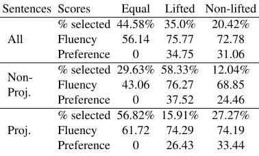
We asked four annotators to judge 60 sentence pairs comparing the lifting-based against the non-lifted linearizer using the toolkit by Kow and Belz (2012). All annotators are students, two of them have a background in linguistics. The items were randomly sampled from the subset of the develop-ment set containing those sentences where the lin-earizers produced different surface realizations. The items are subdivided into 30 originally projective and 30 originally non-projective sentences.

For each item, we presented the original context sentence from the corpus and the pair of automat-ically produced linearizations for the current sen-tence. The annotators had to decide on two crite-ria: (i) which sentence do they prefer? (ii) how flu-ent is that sflu-entence? In both cases, we used con-tinuous sliders as rating tools, since humans seem to prefer them (Belz and Kow, 2011). For the first criterion, the slider positions were mapped to values from -50 (preference for left sentence) to 50 (pref-erence for right sentence). If the slider position is zero, both sentences are equally preferred. For the second criterion, the slider positions were mapped to values from 0 (absolutely broken sentence) to 100 (perfectly fluent sentence).

Sentences Scores Equal Lifted Non-lifted All

% selected 44.58% 35.0% 20.42% Fluency 56.14 75.77 72.78 Preference 0 34.75 31.06

Non-Proj.

% selected 29.63% 58.33% 12.04% Fluency 43.06 76.27 68.85 Preference 0 37.52 24.46

Proj.

% selected 56.82% 15.91% 27.27% Fluency 61.72 74.29 74.19 Preference 0 26.43 33.44 Table 7: Results from human evaluation.

Table 7 presents the results averaged over all sen-tences, as well as for the subsets of non-projective and projective sentences. We report the percentage of items where the judges selected both, the lifted, or non-lifted sentence, alongside with the average

flu-ency score (0-100) and preference strength (0-50). On the entire set of items, the judges selected both sentences in almost half of the cases. However, on the subset of non-projective sentences, the lifted ver-sion is clearly preferred and has a higher average fluency and preference strength. The percentage of zero preference items is much higher on the sub-set of projective sentences. Moreover, the average fluency of the zero preference items is remarkably higher on the projective sentences than on the non-projective subset. We conclude that humans have a strong preference for lifting-based linearizations on non-projective sentences. We attribute the low fluency score on the non-projective zero preference items to cases where the linearizer did not get a cor-rect lifting or could not linearize the lifting corcor-rectly such that the lifted and the non-lifted version were not appropriate. On the other hand, incorrect lift-ings on projective sentences do not necessarily seem to result in deprecated linearizations, which leads to the high percentage of zero preferences with a good average fluency on this subset.

6 Conclusion

We have presented a novel technique to linearize sentences for a range of languages that exhibit projective word order. Our approach deals with non-projectivity by lifting edges in an unordered input tree which can then be linearized by a standard pro-jective linearization algorithm.

We obtain significant improvements for the lifting-based linearization on English, German, Dutch, Danish, Czech and Hungarian, and show that lifting has the largest impact on the V2-languages. In a human evaluation carried out on German we also show that human judges clearly prefer lifting-based linearizations on originally non-projective sentences, and, on the other hand, that incorrect lift-ings do not necessarily result in bad realizations of the sentence.

Acknowledgments

References

A. Belz and E. Kow. 2011. Discrete vs. Continuous Rat-ing Scales for Language Evaluation in NLP. In Pro-ceedings of the 49th Annual Meeting of the Associa-tion for ComputaAssocia-tional Linguistics: Human Language Technologies, pages 230–235, Portland, Oregon, USA, June. Association for Computational Linguistics. A. Belz, M. White, D. Espinosa, D. Hogan, E. Kow, and

A. Stent. 2011. The First Surface Realisation Shared Task: Overview and Evaluation Results. InENLG’11. A. B¨ohmov´a, J. Hajiˇc, E. Hajiˇcov´a, and B. Hladk´a. 2000. The Prague Dependency Treebank: A Three-level an-notation scenario. In A. Abeill´e, editor, Treebanks: Building and using syntactically annotated corpora., chapter 1, pages 103–127. Kluwer Academic Publish-ers, Amsterdam.

B. Bohnet, L. Wanner, S. Mille, and A. Burga. 2010. Broad coverage multilingual deep sentence generation with a stochastic multi-level realizer. InColing 2010, pages 98–106.

B. Bohnet, S. Mille, B. Favre, and L. Wanner. 2011. <stumaba>: From deep representation to surface. In Proceedings of the Generation Challenges Session at the 13th European Workshop on NLG, pages 232–235, Nancy, France.

B. Bohnet. 2004. A Graph Grammar Approach to Map Between Dependency Trees and Topological Models. InIJCNLP, pages 636–645.

N. Br¨oker. 1998. Separating Surface Order and Syntactic Relations in a Dependency Grammar. In COLING-ACL 98.

S. Buchholz and E. Marsi. 2006. CoNLL-X shared task on multilingual dependency parsing. In Proceed-ings of the Tenth Conference on Computational Natu-ral Language Learning, pages 149–164, Morristown, NJ, USA. Association for Computational Linguistics. A. Cahill, M. Forst, and C. Rohrer. 2007. Stochastic

real-isation ranking for a free word order language. ENLG ’07, pages 17–24.

K. Crammer, O. Dekel, S. Shalev-Shwartz, and Y. Singer. 2006. Online Passive-Aggressive Algorithms. Jour-nal of Machine Learning Research, 7:551–585. D. Duchier and R. Debusmann. 2001. Topological

de-pendency trees: A constraint-based account of linear precedence. InProceedings of the ACL.

R. Fan, K. Chang, C. Hsieh, X. Wang, and C. Lin. 2008. LIBLINEAR: A library for large linear classification. Journal of Machine Learning Research, 9:1871–1874. K. Filippova and M. Strube. 2007. Generating con-stituent order in german clauses. InACL, pages 320– 327.

K. Filippova and M. Strube. 2009. Tree linearization in English: improving language model based approaches.

InNAACL, pages 225–228, Morristown, NJ, USA. As-sociation for Computational Linguistics.

M. Gamon, E. Ringger, R. Moore, S. Corston-Olivier, and Z. Zhang. 2002. Extraposition: A case study in German sentence realization. InProceedings of Col-ing 2002. Association for Computational LCol-inguistics. K. Gerdes and S. Kahane. 2001. Word order in german:

A formal dependency grammar using a topological hi-erarchy. InProceedings of the ACL.

Y. Guo, D. Hogan, and J. van Genabith. 2011. Dcu at generation challenges 2011 surface realisation track. InProceedings of the Generation Challenges Session at the 13th European Workshop on NLG, pages 227– 229.

J. Hajiˇc, M. Ciaramita, R. Johansson, D. Kawahara, M.-A. Mart´ı, L. M`arquez, M.-A. Meyers, J. Nivre, S. Pad´o, J. Step´anek, P. Stran´ak, M. Surdeanu, N. Xue, and Y. Zhang. 2009. The CoNLL-2009 shared task: Syntactic and Semantic dependencies in multiple lan-guages. In Proceedings of the 13th CoNLL Shared Task, pages 1–18, Boulder, Colorado.

E. Hajiˇcov´a, J. Havelka, P. Sgall, K. Vesel´a, and D. Ze-man. 2004. Issues of projectivity in the prague de-pendency treebank. Prague Bulletin of Mathematical Linguistics, 81.

W. He, H. Wang, Y. Guo, and T. Liu. 2009. Dependency Based Chinese Sentence Realization. InProceedings of the ACL and of the IJCNLP, pages 809–816. S. Kahane, A. Nasr, and O. Rambow. 1998.

Pseudo-projectivity: A polynomially parsable non-projective dependency grammar. InCOLING-ACL, pages 646– 652.

A. Kathol and C. Pollard. 1995. Extraposition via com-plex domain formation. InMeeting of the Association for Computational Linguistics, pages 174–180. R. Kneser and H. Ney. 1995. InIn Proceedings of the

IEEE International Conference on Acoustics, Speech and Signal Processing, pages 181–184.

E. Kow and A. Belz. 2012. LGRT-Eval: A Toolkit for Creating Online Language Evaluation Experiments. InProceedings of the 8th International Conference on Language Resources and Evaluation (LREC’12). I. Langkilde and K. Knight. 1998. Generation

that exploits corpus-based statistical knowledge. In COLING-ACL, pages 704–710.

J. Nivre and J. Nilsson. 2005. Pseudo-projective de-pendency parsing. InProceedings of the 43rd Annual Meeting of the Association for Computational Linguis-tics (ACL’05), pages 99–106, Ann Arbor, Michigan, June. Association for Computational Linguistics. O. Rambow and A. K. Joshi. 1994. A formal look at

In Leo Wanner, editor,Current Issues in Meaning-Text Theory. Pinter, London, UK.

M. Reape. 1989. A logical treatment of semi-free word order and bounded discontinuous constituency. In Proceedings of the EACL, EACL ’89, pages 103–110. E. Ringger, M. Gamon, R. C. Moore, D. Rojas, M. Smets, and S. Corston-Oliver. 2004. Linguistically informed statistical models of constituent structure for ordering in sentence realization. In COLING ’04, pages 673– 679.

W. Seeker and J. Kuhn. 2012. Making Ellipses Explicit in Dependency Conversion for a German Treebank. In Proceedings of LREC 2012, Istanbul, Turkey. Euro-pean Language Resources Association (ELRA). A. Stent. 2011. Att-0: Submission to generation

chal-lenges 2011 surface realization shared task. In Pro-ceedings of the Generation Challenges Session at the 13th European Workshop on Natural Language Gener-ation, pages 230–231, Nancy, France, September. As-sociation for Computational Linguistics.

V. Vincze, D. Szauter, A. Alm´asi, G. M´ora, Z. Alexin, and J. Csirik. 2010. Hungarian Dependency Tree-bank. In Proceedings of the Seventh conference on International Language Resources and Evaluation (LREC 2010), pages 1855–1862, Valletta, Malta. S. Wan, M. Dras, R. Dale, and C. Paris. 2009. Improving

grammaticality in statistical sentence generation: In-troducing a dependency spanning tree algorithm with an argument satisfaction model. InEACL, pages 852– 860.