Converting Declarative Rules into Decision Trees

Converting Declarative Rules into Decision Trees

Amany Abdelhalim, Issa Traore

Abstract—Most of the methods that generate decision trees for a specific problem use examples of data instances in the decision tree generation process. This paper proposes a method called “RBDT-1”- rule based decision tree -for learning a decision tree from a set of decision rules that cover the data instances rather than from the data instances themselves. RBDT-1 method uses a set of declarative rules as an input for generating a decision tree. The method’s goal is to create on-demand a short and accurate decision tree from a stable or dynamically changing set of rules. We conduct a comparative study of RBDT-1 with existing decision tree methods based on different problems. The outcome of the study shows that in terms of tree complexity (number of nodes and leaves in the decision tree) RBDT-1 compares favorably to AQDT-1, AQDT-2 which are methods that create decision trees from rules. RBDT-1 compares favorably also to ID3 while is as effective as C4.5 where both (ID3 and C4.5) are famous methods that generate decision trees from data examples. Experiments show that the classification accuracies of the different decision trees produced by the different methods under comparison are equal.

Key Words— attribute selection criteria, data-based decision tree , decision rules, rule-based decision tree, tree complexity.

I.INTRODUCTION

Decision Trees are one of the most popular classification algorithms used in data mining and machine learning to create knowledge structures that guide the decision making process. The creation of a good knowledge structure is the main step in the development of a decision making system.

The most common methods for creating decision trees are those that create decision trees from a set of examples (data records). We refer to these methods as data-based decision tree methods.

On the other hand, to our knowledge there are only few approaches that create decision trees from rules proposed in the literature which we refer to as rule-based decision tree methods.

Manuscript received July 23, 2009. A. Abdelhalim is a PHD student in the Electrical and Computer Engineering Department, University of Victoria, P.O.Box 3055 STN CSC,Victoria, B.C., V8W 3P6, Canada, phone: (250) 721-6036, fax:(250)721-6052, e-mail: [email protected]

I. Traore is an Associate Professor and the Coordinator of the Information Security and Object Technology (ISOT) Lab, University of Victoria, Department of Electrical and Computer Engineering., phone:(250)721-8697;fax:(250)721-6052;e-mail: [email protected].

There is a major difference between building a decision tree from examples and building it from rules. When building a decision tree from rules the method assigns attributes to the nodes using criteria based on the properties of the attributes in the decision rules, rather than statistics regarding their coverage of the data examples [1].

A decision tree can be an effective tool for guiding a decision process as long as no changes occur in the dataset used to create the decision tree. Thus, for the data-based decision tree methods once there is a significant change in the data, restructuring the decision tree becomes a desirable task. However, it is difficult to manipulate or restructure decision trees. This is because a decision tree is a procedural knowledge representation, which imposes an evaluation order on the attributes. In contrast, rule-based decision tree methods handle manipulations in the data through the rules induced from the data not the decision tree itself. A declarative representation, such as a set of decision rules is much easier to modify and adapt to different situations than a procedural one. This easiness is due to the absence of constraints on the order of evaluating the rules [2].

On the other hand, in order to be able to make a decision for some situation we need to decide the best order in which tests should be evaluated in those rules. In that case a decision structure (e.g. decision tree) will be created from the rules.

So, rule-based decision tree methods combine the best of both worlds. On one hand they easily allow changes to the data (when needed) by modifying the rules rather than the decision tree itself. On the other hand they take advantage of the structure of the decision tree to organize the rules in a concise and efficient way required to take the best decision. So knowledge can be stored in a declarative rule form and then be transformed (on the fly) into a decision tree only when needed for a decision making situation [2].

In addition to that, generating a decision structure from decision rules can potentially be performed faster than generating it from training examples because the number of decision rules per decision class is usually much smaller than the number of training examples per class. Thus, this process could be done on demand without any noticeable delay [3], [4]. Data-based decision tree methods require examining the complete tree to extract information about any single classification. Otherwise, with rule-based decision tree methods, extracting information about any single classification can be done directly from the declarative rules themselves [1].

by an expert and no data is available, rule-based decision tree methods are the only applicable solution.

This paper presents a new rule-based decision tree method called RBDT-1. To generate a decision tree, the

RBDT-1 method uses in sequence three different criteria to determine the fit (best) attribute for each node of the tree, referred to as the attribute effectiveness (AE), the attribute autonomy (AA), and the minimum value distribution (MVD). In this paper, the RBDT-1 method is compared to the AQDT-1 and AQDT-2 methods which are rule-based decision tree methods, along with the ID3

and C4.5 which are two of the most famous data-based decision tree methods. The attribute selection criteria in

RBDT-1 method give better results than the other methods’ criteria in terms of tree complexity as we show empirically using several publicly available datasets.

The rest of the paper is structured as follows. Section 2 summarizes the related work. Section 3 presents the rule notation and the rule generation method used. Section 4 describes the RBDT-1 method by presenting, in particular, the preparation of the rules into a format that will be used by the method, the different criteria of the method, the decision tree building process, pruning the decision rules and an illustration of the method using a small dataset problem. Section 5 presents the results of an experiment in which, based on public datasets, the proposed method is compared to existing decision tree generation methods. In Section 6, we make some concluding remarks and outline our future work.

II. RELATED WORK

There are few published works on creating decision structures from declarative rules.

The AQDT-1 method introduced in [2] is the first approach proposed in the literature to create a decision tree from decision rules. The AQDT-1 method uses four criteria for selecting the fit attribute that will be placed at each node of the tree. Those criteria are the cost1, the

disjointness, the dominance, and the extent, which are applied in the same specified order in the method’s default setting.

The AQDT-2 method introduced in [1] is a variant of

AQDT-1. AQDT-2 uses five criteria in selecting the fit attribute for each node of the tree. Those criteria are the

cost1, disjointness, information importance, value distribution, and dominance, which are applied in the same specified order in the method’s default setting. In both the AQDT-1&2 methods, the order of each criterion expresses its level of importance in deciding which attribute will be selected for a node in the decision tree. Although both AQDT-1&2 are capable of generating a decision tree from a set of rules, experiments presented in this paper show that our proposed method RBDT-1

produces a less complex tree in most of the cases. Another point is that the calculation of the second criterion - the information importance - in AQDT-2

method depends on the training examples as well as the

1

In the default setting, the cost equals 1 for all the attributes. Thus, the disjointness criterion is treated as the first criterion of the AQDT-1

and AQDT-2 methods in the decision tree building experiments throughout this paper.

rules, which contradicts the method’s fundamental idea of being a rule-based decision tree method. AQDT-2

requires both the examples and the rules to calculate the

information importance at certain nodes where the first criterion- Disjointness - is not enough in choosing the fit attribute. Thus, without the examples, AQDT-2 might not be able to create the decision tree. AQDT-2 being both dependent on the examples as well as the rules increases the running time of the algorithm remarkably in large datasets especially those with large number of attributes.

In contrast the RBDT-1 method, proposed in this work, depends only on the rules induced from the examples, and does not require the presence of the examples themselves. The calculations of the method’s criteria are based on certain characteristics of the attributes intrinsic to the rules only.

Akiba et al. [5] proposed a rule-based decision tree method for learning a single decision tree that approximates the classification decision of a majority voting classifier. Their method was proposed as a possible solution to solve the issues of intelligibility, classification speed, and required space in majority voting classifiers. In their proposed method, if-then rules are generated from each classifier (a C4.5 based decision tree) and then a single decision tree is learned from these rules. Since the final learning result is represented as a single decision tree, problems of intelligibility and classification speed and storage consumption are improved. The procedure that they follow in selecting the best attribute at each node of the tree is based on the C4.5

method which is a data-based decision tree method. The input to the proposed method requires both the real examples used to create the classifiers (decision trees) and the rules extracted from the classifiers, which are used to create a set of training examples to be used in the method.

In [6], the authors proposed a method called Associative Classification Tree (ACT) for building a decision tree from association rules rather than from data. They proposed two splitting algorithms for choosing attributes in the ACT one based on the confidence gain criterion and one based on the entropy gain criterion. The attribute selection process at each node in both splitting algorithms relies on both the existence of rules and the data itself as well. Unlike our proposed method RBDT-1, ACT is not capable of building a decision tree from the rules in the absence of data, or from data (considering them as rules) in the absence of rules.

III. RULE GENERATION AND NOTATIONS

In this section, we present the notations used to describe the rules used by our method. We also present the methods used to generate the rules that will serve as input to the rule-based decision tree methods in our experiments.

A. Notations

Let

a

₁

,...,

a

_ndenote the attributes characterizing the data under consideration, and let

D

₁

,...,

D

_n denote the corresponding domains, respectively (i.e.

D

_i represents the set of values for attribute

a

_i). Let

c

₁

,...,

c

_mrepresent the decision classes associated with the dataset.

The datasets used later in our experiments are based on classification problems where each example in the dataset belongs to only one class. Thus, a desirable form of a rule-set would be a logically disjoint and complete family of rule-sets. Thus, given a collection of rule-sets, one for each class decision, no two rule-sets for two different classes shall logically intersect and the union of all the rule-sets shall cover the whole dataset. In such a case, each possible example in the dataset will belong to one of the predefined classes. So the decision classes induce a partition over the complete set of rules.

B. Rule Generation Method

The RBDT-1 takes rules as input and produces a decision tree as output. Thus, to illustrate our approach and compare it to existing similar approaches, we use in this paper two options for generating a set of disjoint rules for each dataset. The first option is based on extracting rules from a decision tree generated by the ID3 and C4.5 methods, where we convert each branch – from the root to a leaf – of the decision tree to an if-then rule whose condition part is a pure conjunction. This scenario will ensure that we will have a collection of disjoint rules. We refer to these rules as ID3-based rules and C4.5-based rules.

Using ID3-based and C4.5-based rules will give us an opportunity to illustrate our method’s capability of producing a smaller tree while using the same rules extracted from a decision tree generated by a data-based decision tree method without reducing the tree’s accuracy.

The second rule generation option consists of using an

AQ-type rule induction program. AQ-type programs such as AQ19 [7], AQ21 [8], are a family of programs for machine learning and pattern discovery, which are capable of inducing rules from data. In our upcoming experiments we use the AQ19 program for creating logically disjoint rules which we refer to as AQ-based

rules.

IV. RBDT-1 METHOD

In this section, we describe the RBDT-1 method by first outlining the format of the input rules used by the method and the attribute selection criteria of the method. Then we summarize the main steps of the underlying decision tree building process and present the technique used to prune the rules.

A. Preparing the Rules

The decision rules must be prepared into the proper format used by the RBDT-1 method.

This is done by assigning a “don’t care” value to all the attributes that were omitted in any of the rules. The “don’t care” value is equivalent to listing all the values for that attribute. For example, suppose that we have

three attributes

a a

₁

,

₂

and

a

₃with the same domain containing

v v

₁

,

₂

and

v

₃ as possible values.

Let us assume that the following rules correspond to class c1:

r1:c1 a1=v1 & a2=v2, r2: c1 a1=v3

The preparation of these two rules will result in the following formatted rules:

r1: c1 a1=v1 & a2=v2 & a3=”don’t care”,

r2: c1 a1=v3 & a2=”don’t care” & a3=”don’t care”

B. Attribute Selection Criteria

The RBDT-1 method applies three criteria on the attributes to select the fittest attribute that will be assigned to each node of the decision tree. These criteria are the Attribute Effectiveness, the Attribute Autonomy,

andtheMinimum Value Distribution.

Attribute Effectiveness (AE)

AE is the first criterion to be examined for the attributes. It prefers an attribute which has the most influence in determining the decision classes. In other words, it prefers the attribute that has the least number of “don’t care” values for the class decisions in the rules, as this indicates its high relevance for discriminating among rule sets of given decision classes. On the other hand, an attribute which is omitted from all the rules (i.e. has a “don’t care” value) for a certain class decision does not contribute in producing that corresponding decision. So it is considered less important than the other attributes which are mentioned in the rule for producing a decision of that class. Choosing attributes based on this criterion maximizes the chances of reaching leaf nodes faster which on its turn minimizes the branching process and leads to producing a smaller tree.

Using the notation provided above (see section 3), let

ij

V

denote the set of values for attribute

a

_j involved in the rules in

R

_i, which denote the set of rules associated with decision class

c

_i,

1

≤ ≤

i

m

. Let DC denote the ‘don’t care’ value, we calculate

C

_{i j}

(

DC

)

as shown in (1):

1

(

)

0

ij i j

if DC

V

C

DC

otherwise

∈



= 



(1)

Given an attribute

a

_j, where

1

≤ ≤

j

n

, the corresponding attribute effectiveness is given in (2).

1

(

)

(

)

m i j i j

m

C

DC

AE a

m

=

−

=

∑

(2) (Where m is the total number of different classes in the set of rules).

The attribute with the highest AE is selected as the fit attribute.

Attribute Autonomy (AA)

AA is the second criterion to be examined for the attributes. This criterion is examined when the highest AE

criterion prefers the attribute that will decrease the number of subsequent nodes required ahead in the branch before reaching a leaf node. Thus, it selects the attribute that is less dependent on the other attributes in deciding on the decision classes. We calculate the attribute autonomy for each attribute and the one with the highest score will be selected as the fit attribute.

For the sake of simplicity, let us assume that the set of attributes that achieved the highest AE score are

a

₁

,...,

a

_s

, 2

≤ ≤

s

n

. Let ₁

,...,

j

j jp

v

v

denote the set of possible values for attribute

a

_j including the “don’t care”, and

R

_ji denote the rule subsetconsisting of the rules that have

a

_j appearing with the value

v

_ji, where

1

≤ ≤

j

s

and

1

≤ ≤

i

p

_j. Note that

R

_ji will include the rules that have don’t care values for

a

_j as well.

The AA criterion is computed in terms of the Attribute Disjointness Score (ADS), which was introduced by [1]. For each rule subset

R

_ji, let MaxADSji denote the

maximum ADS value and let ADS_Listji denote a list that

contains the ADS score for each attribute

a

_k, where

1

≤ ≤

k

s k

,

≠

j

.

According to [1], given an attribute

a

_jand two

decision classes

c

_i and

c

_k

(where

1

≤

i k

,

≤

m

;1

≤ ≤

j

s

), the degree of disjointness between the rule set for

c

_i and the rule set for

c

_j with respect to attribute

a

_jis defined as shown in (3):

0

1

( , , )

2 ( )

3

if V_ij V_kj

if V_ij V_kj ADS A C C_{j i k}

if V_ij V_kj or V or V_{ij kj}

if V_ij V_kj

⊆

⊇ =

∩ ≠ ∅

∩ =∅















(3)

The Attribute Disjointness of the attribute

a

_j;

( )

j

ADS a score is the summation of the degrees of class

disjointness

ADS a c c

(

_j

, ,

_{i k}

)

given in (4):

1 1

(

)

(

, ,

)

m

j j i k

i k s

i k

ADS a

ADS a c c

= ≤ ≤ ≠

=

∑ ∑

(4)

Thus, the number of ADS_List that will be createdfor each attribute

a

_j as well as the number of MaxADS

values that are calculated will be equal to

p

_j. The

MaxADSji value as defined by [8] is

3

× ×

m

(

m

−

1)

where m is the total number of classes in

R

_ji. We introduce the AA as a new criterion for attribute

a

_j as given in (5):

1

1

(

, )

j

j p

j i

AA (a )

AA a i

=

=

∑

(5)

Where

AA a i

(

_j

, )

is defined as shown in (6):

(

)

( )

₍

₎

(6)

0 0

1

2 0

: [ ]

1 ( 1) [ ]

1

_{if MaxADSji}

if

s

AA (a , i) _{j MaxADS} ji

l MaxADS ADS_List l_{ji ji}

s

s MaxADS_ji ADS_List l otherwise _ji l , l j

=

= ∨ = _{≠ ∧}

∃ =

+ − × − ∑ = ≠





















_

_

_

_













_

_









 



 



 





The AA for each of the attributes is calculated using the above formula and the attribute with the highest AA

score is selected as the fit attribute. According to the above formula,

AA (a , i)

_j equals zero when the class decisions for the rule subset examined corresponds to one class, in that case MaxADS=0, which indicates that a leaf node is reached (best case for a branch).

j

AA (a , i)

equals 1 when s equals 2 or when one of the attributes in the ADS_list has an ADS score equal to

MaxADS value (second best case). The second best case indicates that only one extra node will be required to reach a leaf node.Otherwise

AA (a , i)

_j will be equal to 1 + (the difference between the ADS scores of the attributes in the ADS_list and the MaxADS value) which indicates that more than one node will be required until reaching a leaf node.

Minimum Value Distribution (MVD)

The MVD criterion is concerned with the number of values that an attribute has in the current rules. When the highest AA score is obtained by more than one attribute, this criterion selects the attribute with the minimum number of values in the current rules. MVD criterion minimizes the size of the tree because the fewer the number of values of the attributes the fewer the number of branches involved and consequently the smaller the tree will become [1]. For the sake of simplicity, let us assume that the set of attributes that achieved the highest

AA score are

a

₁

,...,

a

_q

, 2

≤ ≤

q

s

. Given an attribute

a

_j

(where

1

≤ ≤

j

q

), we compute corresponding MVD

value as shown in (7).

1

(

_j

) |

_ij

|

i m

MVD A

V

≤ ≤

=

_∪

(7) (Where |X| denote the cardinality of set X).

where more than two attributes have the lowest MVD

score we take the first attribute.

C. Building the decision tree

In the decision tree building process, we select the fit attribute that will be assigned to each node from the current set of rules CR based on the attribute selection criteria outlined in the previous section. CR is a subset of the decision rules that satisfy the combination of attribute values assigned to the path from the root to the current node. CR will correspond to the whole set of rules at the root node.

From each node a number of branches are pulled out according to the total number of values available for the corresponding attribute in CR.

Each branch is associated with a reduced set of rules

RR which is a subset of CR that satisfies the value of the corresponding attribute. If RR is empty, then a single node will be returned with the value of the most frequent class found in the whole set of rules. Otherwise, if all the rules in RR assigned to the branch belong to the same decision class, a leaf node will be created and assigned a value of that decision class. The process continues until each branch from the root node is terminated with a leaf node and no more further branching is required.

D. Pruning Decision Rules

RBDT-1 is capable of handling the problem of generating a decision tree from noisy training data. In

RBDT-1, we handle noisy data by removing rules that cover only a small portion of the data that could be considered noise [9]. The examples that were covered by the truncated rules can often be covered by applying an analogical matching procedure. The analogical matching procedure determines the degree of similarity between the examples to be classified and the rules of a given decision class, and selects the best matching decision class [10]. In [11] experiments show that such a rule truncation method not only simplifies decision rules which could lead to a simpler decision tree, but could also improve their prediction accuracy in some cases.

In RBDT-1, rules are pruned if their support level is less than or equal to a predefined threshold. The support level of a rule is the percentage of the total number of examples covered by the rule (called the t-weight) to the total number of examples in the given decision class.

[image:5.612.373.506.256.417.2]

Table 1. The weekend rule set induced by AQ19.

Rule# Description

1: Cinema Parents-visiting=”yes” & weather

=”don’t care” & Money =”rich”

2: Tennis Parents-visiting=”no” & weather

=”sunny” & Money =”don’t care”

3: Shopping Parents-visiting=”no” & weather

=”windy” & Money =”rich”

4: Cinema Parents-visiting=”no” & weather

=”windy” & Money =”poor”

5: Stay-in Parents-visiting=”no” & weather

=”rainy” & Money =”poor”

V. ILLUSTRATION OF THE RBDT-1 METHOD In this section the RBDT-1 method is illustrated by a dataset named the weekend problem which is a publicly available dataset.

A. Illustration

The Weekend problem is a dataset that consists of 10 data records obtained from [12]. For this example, we used the AQ19 rule induction program to induce the rule set shown in Table 1 which will serve as the input to our proposed method RBDT-1. AQ19 was used with the mode of generating disjoint rules and with producing a complete set of rules without truncating any of the rules.

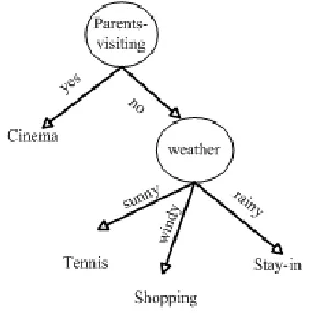
[image:5.612.326.518.534.708.2]

The corresponding decision tree created by the proposed RBDT-1 method for the weekend problem is shown in Figure 1. It consists of 3 nodes and 5 leaves with 100% classification accuracy for the data.

Figure 1. The decision tree generated by RBDT-1 for the weekend problem.

B. Tree Comparison

In this subsection, we present the decision trees generated by the AQDT-1, AQDT-2, ID3 and C4.5

methods for the weekend problem, and compare the outcome trees with that obtained by the RBDT-1 method outlined in the previous section.

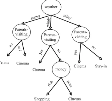
[image:5.612.70.292.587.713.2]

Figure 2 depicts the tree created by AQDT-1&2 and the ID3 methods consisting of 5 nodes and 7 leaves, which is bigger than the decision tree created by the

RBDT-1 method. Both trees have the same classification accuracy as RBDT-1.

As indicated in subsection 4.4, in RBDT-1, rules are pruned if their support level is less than or equal to a predefined threshold. Figure 3 presents a decision tree obtained after pruning the decision rules for the weekend problem in Table 1. In this case, we removed rules with the lowest support level. The produced decision tree by

[image:6.612.115.259.285.428.2]

RBDT-1 misclassified one example out of 10 giving a predictive accuracy of 90% and consists of 2 nodes and 4 leaves.

Figure 4 depicts the decision tree produced by AQDT-1

& 2 using the same pruned rules; although the produced tree has the same accuracy as the tree produced with

RBDT-1, it is bigger in size since it has 4 nodes and 6 leaves. When applying C4.5 to the dataset of the weekend problem it resulted in a tree of the same size and accuracy as RBDT-1 depicted in Figure 3.

Figure 3. The pruned decision tree generated by RBDT-1

for the weekend problem.

Figure 4.The pruned decision tree generated by AQDT-1,

AQDT-2 for the weekend problem.

Due to space limitations, we are unable to include here all of our work. We refer the reader to our extended technical report on RBDT-1 [13] for more details on the decision tree generation and discussion on tree sizes.

VI. EXPERIMENTS

In this section, we present an evaluation of our proposed method by comparing it with the AQDT-1 & 2, the ID3 and the C4.5 methods based on 16 public datasets. Our evaluation consisted of comparing the decision trees produced by the methods for each dataset in terms of tree complexity (number of nodes and leaves) and accuracy. Other than the weekend dataset, all the datasets were obtained from the UCI machine learning repository [14].

We conducted two experiments for comparing RBDT-1

with AQDT-1 &2 and the ID3; the results of these experiments are summarized in Tables 2 and 3. The results in Table 2 are based on comparing the methods using ID3-based rules as input for the rule-based methods. The ID3-based rules were extracted from the decision tree generated by the ID3 method from the whole set of examples of each dataset used. Thus, they cover the whole set of examples (100% coverage). The size of the extracted ID3-based rules is equal to the number of leaves in the ID3 tree.

In Table 3, the experiment was conducted using AQ

-based rules. We used AQ-based rules generated by the

AQ19 rule induction program with 100% correct recognition on the datasets used as input for the rule-based methods under comparison. No pruning is applied by any method in both comparisons presented in Table 2 and 3.

In the following tables, the name of the method that produced a less complex tree appears in the table in the

[image:6.612.80.289.474.617.2]

method column; the “=” symbol indicates that the same tree was obtained by all methods under comparison. All four methods run under the assumption that they will produce a complete and consistent decision tree yielding 100% correct recognition on the training examples.

Table 2. Comparison of tree complexities of the RBDT-1, AQDT-1, AQDT-2 & ID3 methods using ID3-based rules.

Dataset Method Dataset Method

Weekend RBDT-1 MONK’s 1 RBDT-1

Lenses RBDT-1, ID3 MONK’s 2 RBDT-1, AQDT-1 & 2

Chess = MONK’s 3 =

Car RBDT-1, ID3 Zoo =

Shuttle-L-C = Nursery RBDT-1

Connect-4 RBDT-1 Balance RBDT-1, ID3

For 7 of the datasets listed in Table 2, the RBDT-1

produced a smaller tree than that produced by AQDT-1 & 2 with an average of 274 nodes less while producing a same tree for the rest of the datasets. On the other hand,

RBDT-1 produced a smaller tree with 5 of these datasets compared to ID3 with an average of 142.6 nodes less while producing a same tree for the rest of the datasets. The decision tree classification accuracies of all four methods were equal.

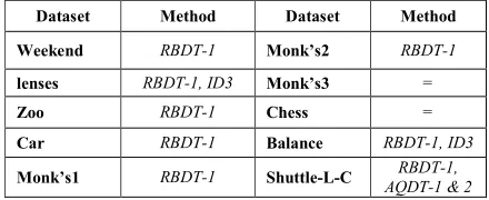
Based on the results of the comparison in Table 3, the

RBDT-1 method performed better than the AQDT-1 & 2

and the ID3 methods in most cases in terms of tree complexity by an average of 33.1 nodes less than AQDT-1 & 2 and by an average of 88.5 nodes less than the ID3

Table 3. Comparison of tree complexities of the RBDT-1, AQDT-1, AQDT-2 & ID3 methods using AQ-based rules.

Dataset Method Dataset Method

Weekend RBDT-1 Monk’s2 RBDT-1

lenses RBDT-1, ID3 Monk’s3 =

Zoo RBDT-1 Chess =

Car RBDT-1 Balance RBDT-1, ID3

Monk’s1 RBDT-1 Shuttle-L-C RBDT-1,

AQDT-1 & 2

We conducted another experiment comparing RBDT-1

to AQDT-1 & 2 and C4.5 using C4.5-based rules. The

C4.5-based rules were extracted from decision trees built by C4.5 method using its default parameters, in the

[image:7.612.69.289.67.157.2]

Orange implementation [15] with the prune option turned “on”.

Table. 4. Comparison of tree complexities of the RBDT-1, AQDT-1, AQDT-2 & C4.5 using C4.5-based rules.

Dataset Method Dataset Method

Weekend RBDT-1, C4.5 MONK’s 1 = Lenses RBDT-1, C4.5 MONK’s 2 =

Chess = MONK’s 3 AQDT-1 & 2

Car RBDT-1, C4.5 Zoo RBDT-1, C4.5

Shuttle-L-C = Breast-C =

Connect-4 RBDT-1, C4.5 Lung-C RBDT-1, C4.5

Nursery = Primary-T RBDT-1, C4.5

Balance = Voting =

The results are summarized in Table 4. The outcome of the comparison is that in terms of tree size, our proposed method RBDT-1 performs better than AQDT-1 & 2 in most of the rule sets. AQDT-1&2 produce a larger tree by an average of 105 nodes with the exception for the

Monk’s3 problem the RBDT-1 tree was only 2 nodes bigger. In addition, the results illustrate that RBDT-1 is as effective as C4.5. In terms of decision tree accuracy, the four methods have equal performance.

VII.CONCLUSIONS AND FUTURE WORK

The RBDT-1 method proposed in this work allows generating a decision tree from a set of rules rather than from the whole set of examples. Following this methodology, knowledge can be stored in a declarative rule form and transformed into a decision structure when it is needed for decision making. Generating a decision structure from decision rules can potentially be performed much faster than by generating it from training examples.

In our experiments, our proposed method was compared to two other rule-based decision tree methods;

AQDT-1 and AQDT-2 using ID3-based rules and AQ-based rules. RBDT-1 was also compared to the ID3 and

C4.5 methods which are data-based decision tree methods. Based on the results of the comparison the

RBDT-1 method performs better than the other three methods under comparison in most cases in terms of tree complexity and achieves at least the same level of accuracy. It appears also that RBDT-1 performs equally well as C4.5.

In our future work we will conduct more experiments using rule sets produced by different methods of rule generation. We will also extend our method to address the

problem of learning from rules that do not logically intersect.

ACKNOWLEDGMENTS

The authors would like to thank the UCI machine learning repository for the datasets used in the presented experiments. We also thank Dr. Janusz Wojtusiak the director of the Machine Learning and Inference Laboratory at George Mason University [http://www.mli.gmu.edu] for providing us with the

AQ19 rule inductionprogram.

REFERENCES

[1] R. S. Michalski and I. F. Imam, “Learning problem-oriented decision structures from decision rules: the AQDT-2 system”, In Proceedings of 8th International Symposium Methodologies for Intelligent Systems. Lecture Notes in Artificial Intelligence, 869, Springer Verlag, Heidelberg, 1994, pp. 416-426.

[2] Imam, I. F., and R. S. Michalski. “Should decision trees be learned from examples of from decision rules?”, Source Lecture Notes in Computer Science. In Proceedings of the 7th

International Symposium on Methodologies, 689, 1993, pp. 395–404. [3] J. R. Quinlan, “Discovering rules by induction from large

collections of examples”, In D. Michie (Edr), Expert Systems in the Microelectronic Age, Edinburgh University Press, 1979, pp. 168-201.

[4] I. H. Witten, and B. A. MacDonald. “Using concept learning for knowledge acquisition”, International Journal of Man-Machine Studies, 1988, pp. 349-370.

[5] Y. Akiba,, S. Kaneda, and H. Almuallim, “Turning majority voting classifiers into a single decision tree”, In Proceedings of the 10th IEEE International Conference on Tools with Artificial Intelligence, 1998, pp. 224-230.

[6] Y. Chen, L. T. Hung,” Using decision trees to summarize associative classification rules”. Expert Syst. Appl. Pergamon Press, Inc. Publisher, 2009, 36(2): pp. 2338--2351

[7] R. S. Michalski, and K. Kaufman. “The aq19 system for machine learning and pattern discovery: a general description and user's guide”, Reports of the Machine Learning and Inference Laboratory, MLI 01-2, George Mason University, Fairfax, VA, 2001.

[8] J. Wojtusiak, “AQ21 user’s guide”. Reports of the Machine Learning and Inference Laboratory, MLI 04-5, George Mason University, 2004.

[9] R. S. Michalski, I. F. Imam, “On learning decision structures”. fundamenta informaticae, 1997, 31(1): pp. 49--64

[10] Michalski, R.S., Mozetic, I., Hong, J., Lavrac, N.: The Multi-Purpose Incremental Learning System AQ15 and its Testing Application to Three Medical Domains. In: Proceedings of AAAI-86, Philadelphia, PA, 19AAAI-86, pp. 1041--1045

[11] F. Bergadano, S. Matwin, R. S. Michalski, J. Zhang, “Learning two-tiered descriptions of flexible concepts: the POSEIDON system”. Machine Learning, 1992, Vol. 8, No. 1, pp. 5--43 [12] Colton, S. Online Document, Available:

http://www.doc.ic.ac.uk/~sgc/teaching/v231/lecture11.html. 2004. [13] A. Abdelhalim and I. Traore, “The RBDT-1 Method for

Rule-based Decision Tree Generation”, Technical report #ECE-09-1, ECE Department, University of Victoria, PO Box 3055, STN CSC, Victoria, BC, Canada, July 2009.

[14] A. Asuncion, and D.J. Newman, UCI Machine Learning Repository [http://www.ics.uci.edu/~mlearn/MLRepository.html]. Irvine, CA: University of California, School of Information and Computer Science, 2007.