How Well Can We Predict Hypernyms from Word Embeddings? A Dataset Centric Analysis

How Well Can We Predict Hypernyms from Word Embeddings?

A Dataset-Centric Analysis

V. Ivan Sanchez Carmona and Sebastian Riedel University College London

Department of Computer Science

{i.sanchezcarmona, s.riedel}@cs.ucl.ac.uk

Abstract

One key property of word embeddings currently under study is their capacity to encode hypernymy. Previous works have used supervised models to recover hyper-nymy structures from embeddings. How-ever, the overall results do not clearly show how well we can recover such struc-tures. We conduct the first dataset-centric analysis that shows how only the Baroni dataset provides consistent results. We empirically show that a possible reason for its good performance is its alignment to di-mensions specific of hypernymy: general-ityandsimilarity.

1 Introduction

Word embeddings have been widely used as fea-tures in NLP tasks like parsing and textual entail-ment. One key aspect that has been investigated is their capacity to encode hypernymy; this semantic relation denotes a taxonomical order of objects in the world; for example, a dogis a canine which

is a vertebrate. To test the ability of embeddings to encode hypernymy, previous work has proposed supervised models to learn whether a given pair of embeddings (wi, wj) are in the hypernymy

rela-tion (Roller et al., 2014; Necsulescu et al., 2015; Fu et al., 2014).

Results from previous work suggest that word embeddings indeed capture hypernymy informa-tion. This observation is relatively general and robust across several choices of datasets, mod-els and embeddings. For example, Levy et al. (2015) achieve up to 0.85 F1, while Roller and Erk (2016) achieve up to 0.90 F1. Both of these results are achieved on the Baroni dataset (Baroni et al., 2012). For most other datasets, models achieve promising scores above 0.60 F1 points; e.g. Roller

and Erk (2016) report 0.66 F1 points for a linear model on the balanced Turney dataset (Turney and Mohammad, 2015).

On closer look, however, we find that the cur-rent F1-based results may be somewhat mislead-ing. In particular, several papers report F1 scores in the higher 60% level onbalanceddatasets—on such datasets a baseline that predicts each pair to be in the hypernym relation already achieves 66% F1. And when calculating accuracy instead of F1 scores we observe accuracies around 50%-60% for state of the art models, often barely above chance level (Table 3).

There is one striking exception when it comes to accuracy results. On the Baroni dataset, accu-racy is as high as 81%. These observations lead us to the following questions regarding the datasets and overall results: Are the scores on the Baroni dataset high because it is aneasydataset? Or are they high because it is easier to learn hypernymy from the Baroni training set due to its design? To what extent can the Baroni dataset help us to pre-dict hypernyms from word embeddings?

In this work we conduct the first dataset-centric analysis across 6 datasets to empirically answer the questions above. We take inspiration from the work of (Torralba and Efros, 2011) in the com-puter vision domain where a set of datasets are compared and biases are exposed. In the same spirit, we compare a set of datasets by evaluating the ability of models trained on such datasets to generalize to different test distributions.

We show how the Baroni dataset outperforms the other datasets. In particular, we find that mod-els trained on Baroni’s data can outperform other models even on their home turf. For example, a model trained on Baroni’s data can do better on the Kotlerman (Kotlerman et al., 2010) test set than models trained on the Kotlerman training set with the same size.

Furthermore, we show that the Baroni dataset seems to exhibit a pronounced behaviour along two dimensions known to be relevant for hyper-nymy: generalityand similarity. This behaviour appears to be important for the success of Baroni’s dataset: if we filter and resample other training datasets with respect to this behaviour, we gener-ally achieve better results.

2 Background

We first give a brief overview of hypernymy detec-tion, important findings in this domain, and then relevant work on dataset analysis.

2.1 Supervised Hypernym Detection

The task is posed as a binary classification prob-lem. An instance pair is composed of two em-beddings, e.g. (wcat, wanimal,positive). A vector

operation such as concatenation (concat) or dif-ference (diff) is then applied to both embeddings. Vylomova et al. (2016) learned a range of seman-tic relations, including hypernymy, using the diff

operator and achieved positive results. Roller and Erk (2016) showed thatconcatwith a logistic re-gression classifier learns to extract Hearst patterns (such as,including, etc.) from distributional vec-tors.

Weeds et al. (2014) and Vylomova et al. (2016) described the lexical memorizationphenomenon: a classifier learns that a word wi is hyponym of

a word wj based on the frequency of wj

appear-ing in the hypernym slot in positive pairs. In order to avoid high scores at test time due to this effect, Weeds et al. (2014) suggest having disjoint vocab-ularies between training and test sets.

2.2 Dataset Analysis

Torralba and Efros (2011) compared a set of ob-ject recognition datasets by testing each of them across different test distributions. In order to fairly compare these datasets, Torralba and Efros (2011) first eliminated some visible biases such as sample size by normalizing the datasets. In this way, other biases in the datasets were exposed such as the photographer’s shooting position, or the labellers’ perception, that may not be easily observable and may harm the classifier performance. Torralba and Efros (2011) concluded that some datasets are a better representation of the problem domain.

3 Materials

We describe both the datasets that we compare and the word embedding model that we use as features.

3.1 Datasets

We pick the datasets used by Levy et al. (2015) and Weeds et al. (2014) which have disjoint training and test sets.

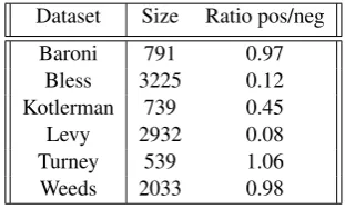
Dataset Size Ratio pos/neg Baroni 791 0.97

Bless 3225 0.12 Kotlerman 739 0.45 Levy 2932 0.08 Turney 539 1.06 Weeds 2033 0.98

Table 1: Summary of datasets.

BaroniBaroni et al. (2012) drew instance pairs from WordNet that were manually checked to dis-card noisy ones.

Bless The original dataset (Baroni and Lenci, 2011) contains several semantic relations. Levy et al. (2015) used the hypernymy pairs as positive instances and the pairs in all the other semantic relations as negative instances.

KotlermanKotlerman et al. (2010) adapted the lexical entailment dataset of (Zhitomirsky-Geffet and Dagan, 2009).

LevyFrom a set of entailing propositions of the form(subject, verb, object)in (Levy et al., 2014), Levy et al. (2015) extracted entailing nouns that shared two arguments to create instance pairs.

Turney Turney and Mohammad (2015) trans-formed the SemEval-2012 dataset (Jurgens et al., 2012) to expand from 79 to 158 semantic relations.

WeedsWeeds et al. (2014) drew instance pairs from WordNet under the constraint that none of the words in a pair must be seen in any other pair in the same role (hyponym or hypernym).

3.2 Word Embeddings

We pick what we believe to be one of the most representative word embedding models.

GloVe Pennington et al. (2014) designed a vec-tor space model using a log-bilinear regression function. They learned unsupervised word embed-dings from a matrix of word co-ocurrences while maintaining linear sub-structures in such space.

4 Cross-test Evaluation

We evaluate the robustness of the six datasets for generalising to different test distributions. In or-der to fairly compare the datasets, we follow Tor-ralba and Efros (2011) and remove biases such as sample size and imbalance by sub-sampling with replacement and uniformly at random the training sets. We obtain 20 subsets, i.e. samples, from each of the training sets. Each sample is normalized and balanced to 400 instances.1

We learn a model for each sample using the Scikit-learn (Pedregosa et al., 2011) package and test it on all the six test sets. We try all combi-nations of vector operator (diff,concat) and clas-sifier (logistic regression, SVM). Hyperparameter tuning and model selection are performed using self-validation sets. We report AUC and accuracy scores solely for the Glove embeddings of dimen-sionality 50 given that the results on other embed-ding models are quite comparable.

4.1 Ranking Pairs: AUC ROC

The Area Under the ROC Curve measures the ability of a classifier to rank positive instances with respect to negative ones independently of any threshold value. Unfortunately, this metric may throw an overoptimistic value under highly imbal-anced data: a disproportional number of negative instances will push the positive ones higher in the ranking, while false positives will slightly affect the overall score (Zou et al., 2016). Therefore we balance the test sets using an under-sampling scheme.2

In Table 2 we can see that, remarkably, the Ba-roni dataset surpasses all datasets on their own self-test sets, except for the Bless test. Interest-ingly, all the training sets performed better on the Baroni test set than on their self-test set (except, for the Bless dataset). This indicates both the ro-bust generalization and superior performance of the Baroni dataset.3

We note that no training sample has overlap with any self or cross test set, except for the Weeds dataset. On the one hand, the Weeds training

sam-1_{We sample 200 positive instances since that is the}

mini-mum number of positives found in any of the datasets.

2_{We also try an oversampling scheme, but the results are}

comparable.

3_{We find that the combination of SVM classifier with RBF}

kernel and diff vector operator gives the best performance on validation set for all the 20 samples drawn from Baroni training set.

ples slightly overlap with the cross-test sets. On the other hand, the Weeds test set overlaps in at least 10% of the pairs with the cross-training sam-ples. This may influence the cross-test scores (Vy-lomova et al., 2016).

4.2 Detecting Hypernyms: Accuracy

We optimize a threshold, on self-validation sets, for each model in Section 4.1. In Table 3 we can see again the superior performance of the Baroni dataset. While the mean of all the self-test scores (main diagonal) is 0.606 points, Baroni achieves a mean of 0.655 points.

Interestingly, in average all the datasets perform close to a random behavior, with the exception of the Baroni and Weeds datasets.4 _Furthemore,

this poor behavior is observed on self-test sets for 3 datasets (Kotlerman, Levy, and Turney). This contrasts to the AUC scores obtained before. One possible cause may be a sensitivity problem in the threshold optimization.

5 Dataset Analysis

We provide an empirical rationale behind the good performance of the Baroni dataset: we believe it aligns to two dimensions specific of hypernymy – generality and similarity– i.e. the instances in the dataset form what we believe to be patterns denot-ing hypernymy. We explain below these patterns.

We use WordNet (Fellbaum, 1998) to com-pute both generality and similarity levels. We de-fine generality levels as the absolute difference, in number of edges, of two words to the root of the taxonomy: g = |distance(word1, root) − distance(word2, root)|. We define similarity

lev-els as the similarity score between two words; we use the Wu-Palmer function.5

We explain now the patterns mentioned above. In the generality levelg= 0, where co-hyponyms exist, we expect only negative pairs to populate the dataset. In the rest of the levels, we would expect a distribution where the number of instance pairs is inversely proportional to the generality level be-cause the branching factor at the bottom levels is greater by a factorαin comparison to the top lev-els; this means that we are more likely to sam-ple pairs of words connected by fewer number of

4_{However, recall that as noted in Sec. 4.1, Weeds scores}

on cross-test results may be influenced by lexical memoriza-tion issues.

5_{We re-scale from [0.0,1.0] to [-1.0,1.0] for visualization}

Train Test Baroni Bless Kotlerman Levy Turney Weeds Mean Baroni 0.916 0.711 0.616 0.702 0.654 0.686 0.714 Bless 0.762 0.850 0.555 0.632 0.600 0.615 0.669 Kotlerman 0.653 0.612 0.543 0.566 0.581 0.544 0.583 Levy 0.716 0.611 0.592 0.698 0.569 0.533 0.619 Turney 0.686 0.646 0.547 0.595 0.646 0.520 0.606 Weeds 0.817 0.645 0.574 0.687 0.637 0.675 0.672

Table 2: Cross-test performance: Mean AUC scores over 20 samples. Self-test score in bold.

Train Test Baroni Bless Kotlerman Levy Turney Weeds Mean Baroni 0.812 0.638 0.587 0.653 0.608 0.636 0.655 Bless 0.578 0.642 0.505 0.526 0.524 0.508 0.547 Kotlerman 0.563 0.546 0.520 0.524 0.528 0.528 0.534 Levy 0.521 0.510 0.507 0.522 0.509 0.496 0.510 Turney 0.546 0.534 0.518 0.540 0.540 0.479 0.526 Weeds 0.736 0.579 0.553 0.626 0.599 0.600 0.615

Table 3: Cross-test performance: Mean accuracy scores over 20 samples. Self-test score in bold.

edges than by higher number of edges.

On the other hand, for the similarity distribu-tion, as a function of the number of edges, at large values we expect a dominance of positive in-stances because the number of edges between the words in a true hypernym pair is generally fewer than between a non-hypernym pair. In addition, as we argued for the generality distribution, we are more likely to sample shorter hypernym pairs than longer pairs.

5.1 Exploring the Baroni dataset

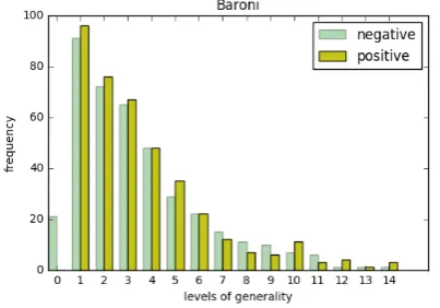
In Fig. 1 we see that at level g = 0only nega-tive pairs are found in the Baroni dataset. We also observe that the distribution matches the expected distribution along generality levels. In Fig. 2 we see that from the levels = 0.2, towards the high-est levels, there is a clear dominance of positive pairs; though we also find negative pairs in these levels. These negative pairs may be positive pairs reversed, e.g. (wanimal, wcat, negative), or pairs

withrelatedwords, e.g. (wcat, winvertebrate,

neg-ative). We also see that from the level s = 0.1

towards the lowest levels, the negative pairs dom-inate.

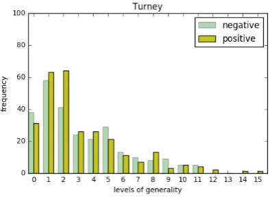
We compare the Baroni distribution with the Turney distribution. In Fig. 3 we observe that the shape of the generality distribution roughly fits our expected distribution; however, we see that pos-itive pairs populate level g = 0. This seems to show that around 10% of the positive pairs in the

Turney dataset are spurious pairs.

In Fig. 4 we observe that the similarity distri-bution from the Turney dataset does not fit the ex-pected distribution. Even though at high levels the dominance is mainly of positive pairs, at low lev-els we also see a strong presence of positive pairs along with negative pairs. This may imply that a high number of positive pairs are noisy or incon-sistent, which may explain the low performance of the Turney dataset.

Figure 1: Distribution of instance pairs on the Ba-roni dataset along generality levels.

5.2 Mimicking the Baroni Distribution

Train Test Baroni Bless Kotlerman Levy Turney Weeds Mean New train set 0.794(0.05) 0.664(0.02) 0.580(0.03) 0.644(0.02) 0.596(0.02) 0.629(0.03) 0.651 Baseline 0.775(0.06) 0.655(0.02) 0.566(0.03) 0.641(0.02) 0.596(0.02) 0.598(0.03) 0.638

Table 4: New dataset vs. Baseline: Mean accuracy scores and standard deviation over 20 samples.

Figure 2: Distribution of instance pairs on the Ba-roni dataset along similarity levels.

Figure 3: Distribution of instance pairs on the Tur-ney dataset along generality levels.

training sets such that we mimic the Baroni distri-butions in Fig. 1 and Fig. 2. More specifically, we allow a pair to populate our new training set if it fulfils constraints regarding the number of in-stances along generality and similarity levels.

One example constraint that needs to be fulfilled for positive pairs is: IF generality level g > 0

AND positive vs. negative pairs ratio is fulfilled according to ratiorg AND similarity levels >=

0.1 AND positive vs. negative pairs ratio is ful-filled according to ratiorsTHEN accept pair.

We obtain 20 balanced and normalized samples populated with 400 instances in each of them. We compare against a dataset baseline where we allow any pair, chosen uniformly at random, to populate

Figure 4: Distribution of instance pairs on the Tur-ney dataset along similarity levels.

the baseline. For building the dataset baseline, we use the same random seeds as those used for build-ing the samples that mimic the Baroni distribution. In Table 4 we see how the new training set robustly outperforms the baseline. These results support our hypothesis for why the Baroni dataset is able to outperform all the datasets.

6 Conclusions

We performed the first dataset-centric analysis for investigating how well we can predict hypernym pairs from word embeddings. We showed in cross-test evaluations how –in contrast to what results from previous work suggest– the Baroni dataset is the only one that consistently enables us to predict hypernym pairs. We empirically showed that the superior performance of the Baroni dataset may be in part due to its alignment to two dimensions relevant to of hypernymy: generality and simi-larity. We empirically corroborated this hypoth-esis by building a new training set that mimics the Baroni distribution and outperforms on average a dataset baseline.

Acknowledgments

References

Marco Baroni and Alessandro Lenci. 2011. How we blessed distributional semantic evaluation. In Pro-ceedings of the GEMS 2011 Workshop on GEomet-rical Models of Natural Language Semantics, pages 1–10. Association for Computational Linguistics. Marco Baroni, Raffaella Bernardi, Ngoc-Quynh Do,

and Chung-chieh Shan. 2012. Entailment above the word level in distributional semantics. In Proceed-ings of the 13th Conference of the European Chap-ter of the Association for Computational Linguistics, pages 23–32, Avignon, France, April. Association for Computational Linguistics.

Christiane Fellbaum. 1998. WordNet: An Electronic Lexical Database. MIT Press., Cambridge, MA. Ruiji Fu, Jiang Guo, Bing Qin, Wanxiang Che, Haifeng

Wang, and Ting Liu. 2014. Learning semantic hier-archies via word embeddings. InProceedings of the 52nd Annual Meeting of the Association for Compu-tational Linguistics (Volume 1: Long Papers), pages 1199–1209, Baltimore, Maryland, June. Association for Computational Linguistics.

David Jurgens, Saif Mohammad, Peter Turney, and Keith Holyoak. 2012. Semeval-2012 task 2: Mea-suring degrees of relational similarity. In *SEM 2012: The First Joint Conference on Lexical and Computational Semantics – Volume 1: Proceedings of the main conference and the shared task, and Vol-ume 2: Proceedings of the Sixth International Work-shop on Semantic Evaluation (SemEval 2012), pages 356–364, Montr´eal, Canada, 7-8 June. Association for Computational Linguistics.

Lili Kotlerman, Ido Dagan, Idan Szpektor, and Maayan Zhitomirsky-Geffet. 2010. Directional distribu-tional similarity for lexical inference. Natural Lan-guage Engineering, 16(04):359–389.

Omer Levy, Ido Dagan, and Jacob Goldberger. 2014. Focused entailment graphs for open ie propositions. In Proceedings of the Eighteenth Conference on Computational Natural Language Learning, pages 87–97, Ann Arbor, Michigan, June. Association for Computational Linguistics.

Omer Levy, Steffen Remus, Chris Biemann, and Ido Dagan. 2015. Do supervised distributional meth-ods really learn lexical inference relations? In Pro-ceedings of the 2015 Conference of the North Amer-ican Chapter of the Association for Computational Linguistics: Human Language Technologies, pages 970–976, Denver, Colorado, May–June. Association for Computational Linguistics.

Silvia Necsulescu, Sara Mendes, David Jurgens, N´uria Bel, and Roberto Navigli. 2015. Reading between the lines: Overcoming data sparsity for accurate classification of lexical relationships. In Proceed-ings of the Fourth Joint Conference on Lexical and Computational Semantics, pages 182–192, Denver,

Colorado, June. Association for Computational Lin-guistics.

F. Pedregosa, G. Varoquaux, A. Gramfort, V. Michel, B. Thirion, O. Grisel, M. Blondel, P. Pretten-hofer, R. Weiss, V. Dubourg, J. Vanderplas, A. Pas-sos, D. Cournapeau, M. Brucher, M. Perrot, and E. Duchesnay. 2011. Scikit-learn: Machine learn-ing in Python. Journal of Machine Learning Re-search, 12:2825–2830.

Jeffrey Pennington, Richard Socher, and Christopher Manning. 2014. Glove: Global vectors for word representation. In Proceedings of the 2014 Con-ference on Empirical Methods in Natural Language Processing (EMNLP), pages 1532–1543, Doha, Qatar, October. Association for Computational Lin-guistics.

Stephen Roller and Katrin Erk. 2016. Relations such as hypernymy: Identifying and exploiting hearst pat-terns in distributional vectors for lexical entailment. In Proceedings of the 2016 Conference on Empiri-cal Methods in Natural Language Processing, pages 2163–2172, Austin, Texas, November. Association for Computational Linguistics.

Stephen Roller, Katrin Erk, and Gemma Boleda. 2014. Inclusive yet selective: Supervised distributional hy-pernymy detection. In Proceedings of COLING 2014, the 25th International Conference on Compu-tational Linguistics: Technical Papers, pages 1025– 1036, Dublin, Ireland, August. Dublin City Univer-sity and Association for Computational Linguistics. Antonio Torralba and Alexei A. Efros. 2011. Unbiased look at dataset bias. InComputer Vision and Pat-tern Recognition (CVPR), 2011 IEEE Conference on, pages 1521–1528. IEEE.

Peter D. Turney and Saif M. Mohammad. 2015. Ex-periments with three approaches to recognizing lex-ical entailment. Natural Language Engineering, 21(03):437–476.

Ekaterina Vylomova, Laura Rimell, Trevor Cohn, and Timothy Baldwin. 2016. Take and took, gaggle and goose, book and read: Evaluating the utility of vector differences for lexical relation learning. In

Proceedings of the 54th Annual Meeting of the As-sociation for Computational Linguistics (Volume 1: Long Papers), pages 1671–1682, Berlin, Germany, August. Association for Computational Linguistics. Julie Weeds, Daoud Clarke, Jeremy Reffin, David Weir, and Bill Keller. 2014. Learning to distinguish hy-pernyms and co-hyponyms. InProceedings of COL-ING 2014, the 25th International Conference on Computational Linguistics: Technical Papers, pages 2249–2259, Dublin, Ireland, August. Dublin City University and Association for Computational Lin-guistics.

Maayan Zhitomirsky-Geffet and Ido Dagan. 2009. Bootstrapping distributional feature vector quality.