A single input single output formulation for yaw rate and sideslip angle control via torque vectoring

A single input single output formulation for yaw rate and

sideslip angle control via torque-vectoring

LENZO, Basilio <http://orcid.org/0000-0002-8520-7953>, SORNIOTTI, Aldo

and GRUBER, Patrick

Available from Sheffield Hallam University Research Archive (SHURA) at:

http://shura.shu.ac.uk/21370/

This document is the author deposited version. You are advised to consult the

publisher's version if you wish to cite from it.

Published version

LENZO, Basilio, SORNIOTTI, Aldo and GRUBER, Patrick (2018). A single input

single output formulation for yaw rate and sideslip angle control via torque-vectoring.

In: 14th Symposium on Advanced Vehicle Control, Beijing, 16-20 July 2018. (In

Press)

Copyright and re-use policy

See http://shura.shu.ac.uk/information.html

Sheffield Hallam University Research Archive

A Single Input Single Output Formulation for Yaw Rate and

Sideslip Angle Control via Torque-Vectoring

Basilio Lenzo

_{, Aldo Sorniotti}

_{, Patrick Gruber}

1

_{Department of Engineering and Mathematics, Sheffield Hallam University, S1 1WB}

Sheffield, UK

2

_{Centre for Automotive Engineering, University of Surrey, GU2 7XH Guildford, UK}

E-mail: [email protected]

Many torque-vectoring controllers are based on the concurrent control of yaw rate and sideslip angle through complex multi-variable control structures. In general, the target is to continuously track a reference yaw rate, and constrain the sideslip angle to remain within thresholds that are critical for vehicle stability. To achieve this objective, this paper presents a single input single output (SISO) formulation, which varies the reference yaw rate to constrain sideslip angle. The performance of the controller is successfully validated through simulations and experimental tests on an electric vehicle prototype with four drivetrains.

Topics / Vehicle Dynamics and Chassis Control

1. INTRODUCTION

Electric vehicles with individually controlled drivetrains provide significant benefits in terms of active safety and drivability. In fact, they allow the allocation of desired amounts of torque to each driven wheel, i.e., torque-vectoring (TV). TV permits the generation of a direct yaw moment through the controlled left-to-right wheel torque distribution. TV has been widely investigated in the literature. Several studies propose TV-based yaw rate control strategies to improve vehicle handling [1-4], shape the vehicle understeer characteristic, and increase yaw and sideslip damping during transients [5-7]. Vehicle handling is also influenced by the variation of the front-to-rear wheel torque distribution, which is achievable in four-wheel-drive vehicles with TV capability [8-9].

Yaw rate controllers need the generation of a reference yaw rate, requiring a good estimation of the tire-road friction coefficient [10]. TV controllers using a reference yaw rate based on inaccurate friction estimation can lead to dangerous vehicle behavior (see [11-12] for general discussions on the topic). However, prompt friction estimation is still a difficult task. Therefore, the yaw rate controller can be coupled with an appropriate sideslip angle controller, able to provide safe performance at the vehicle cornering limit, even in presence of rather imprecise friction estimation [13].

This paper presents a single input single output (SISO) formulation for concurrent yaw rate and sideslip angle control. The reference yaw rate is varied as a function of the estimated or measured sideslip angle. The formulation is validated via phase-plane simulations and experiments on an electric vehicle prototype.

2. CONTROLLER

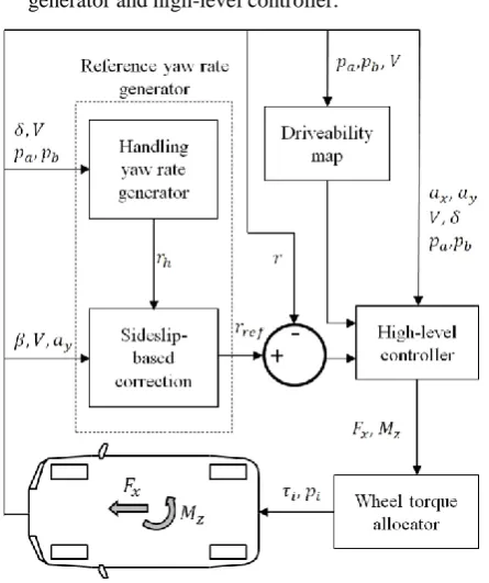
The simplified schematic of the vehicle control

structure is shown in Fig. 1 [12]. It includes:

 A reference yaw rate generator, consisting of two sub-systems. The "Handling yaw rate generator" defines the so-called handling yaw rate, 𝑟ℎ , which

corresponds to a desired vehicle cornering response in steady-state conditions, assuming a certain tire-road friction level. In the "Sideslip-based correction" sub-system, 𝑟_ℎ is corrected based on the actual sideslip angle and lateral acceleration, as detailed later.

 A high-level controller, generating the overall traction/braking force and direct yaw moment demands, respectively 𝐹𝑋 and 𝑀𝑍, to achieve the

reference vehicle behavior, starting from the outputs of the drivability maps and reference yaw rate generator. In this study 𝑀𝑍 is the output of a

proportional integral (PI) controller, such as the one in [6]. However, the proposed formulations and analyses have general validity, and could be implemented with any other SISO control structure.

 A wheel torque allocator, which calculates the reference motor torques, 𝜏𝑖, and brake pressures, 𝑝𝑖,

for each wheel, to generate the values of 𝐹𝑋 and 𝑀𝑍

requested by the high-level controller. The total drivetrain torques on the left- and right-hand sides of the vehicle, 𝜏𝐿 and 𝜏𝑅, are obtained as:

𝜏𝐿= 0.5 (𝐹𝑋−

𝑀𝑍

𝑑) 𝑅𝑤 𝜏𝑅= 0.5 (𝐹𝑋+

𝑀𝑍

𝑑 ) 𝑅𝑤

(1)

where 𝑑 is the half-track width and 𝑅𝑤 is the wheel

However, a simple and predictable control allocation algorithm is ideal for the analysis of this study, focused on the performance of the reference yaw rate generator and high-level controller.

Fig. 1. Simplified control structure schematic (from [12]). In the proposed formulation, a first order transfer function is adopted to calculate the reference yaw rate,

𝑟𝑟𝑒𝑓, from its steady-state value, 𝑟𝑟𝑒𝑓,𝑠𝑡, which is given

by:

𝑟𝑟𝑒𝑓,𝑠𝑡= 𝑟ℎ− 𝐹(𝑟ℎ− 𝐾𝑠𝑟𝑠)

= (1 − 𝐹)𝑟ℎ+ 𝐹𝐾𝑠𝑟𝑠

(2) where 𝑟ℎ is the handling yaw rate; 𝑟𝑠 is the stability yaw

rate, i.e., a yaw rate that is compatible with the current cornering conditions of the vehicle, corresponding to the measured lateral acceleration, 𝑎𝑦 ; and 𝐹 is a linear

function of the absolute value of the sideslip angle, |𝛽|, saturated between 0 and 𝐾𝑓:

𝐹 =

{

0 𝑖𝑓 |𝛽| < 𝛽𝑎𝑐𝑡

|𝛽| − 𝛽𝑎𝑐𝑡

𝛽𝑙𝑖𝑚− 𝛽𝑎𝑐𝑡𝐾𝑓 𝑖𝑓 𝛽𝑎𝑐𝑡 ≤ |𝛽| ≤ 𝛽𝑙𝑖𝑚

𝐾𝑓 𝑖𝑓 |𝛽| > 𝛽𝑙𝑖𝑚

(3)

The sideslip-based correction intervenes only when

|𝛽| is beyond the activation threshold, 𝛽𝑎𝑐𝑡 . This

threshold is sufficiently large such that it is not exceeded during the normal operation of the yaw rate controller in high friction conditions. On the other hand, a sideslip angle exceeding 𝛽𝑎𝑐𝑡 indicates a too high yaw rate. If |𝛽|

is above the limit threshold, 𝛽𝑙𝑖𝑚 , the sideslip-based

contribution reduces the reference yaw rate to 𝑟𝑟𝑒𝑓,𝑠𝑡=

(1 − 𝐾𝑓)𝑟ℎ+ 𝐾𝑓𝐾𝑠𝑟𝑠. For example, if the tuning

parameters 𝐾𝑓 and 𝐾𝑠 are assumed equal to 1, then

𝑟𝑟𝑒𝑓,𝑠𝑡= 𝑟𝑠 for high values of sideslip angle. This

approach is simpler and easier to tune compared to [16], which also takes into account the sideslip angle rate, 𝛽̇.

𝑟𝑠 is calculated from its saturation value, 𝑟𝑠𝑎𝑡, which is a

function of 𝑎𝑦 according to the steady-state relationship

between yaw rate and 𝑎𝑦 [12]:

𝑟𝑠𝑎𝑡 =

𝑎𝑦− 𝑠𝑖𝑔𝑛(𝑎𝑦)𝛥𝑎𝑦

𝑉 (4)

The parameter 𝛥𝑎𝑦 , which varies as a function of 𝑎𝑦 ,

ensures that the vehicle with a yaw rate equal to 𝑟𝑠𝑎𝑡 is

actually operating within its cornering limit. 𝑟𝑠 is given

by:

𝑟𝑠 = {_|𝑟 𝑟ℎ 𝑖𝑓 |𝑟ℎ| < |𝑟𝑠𝑎𝑡|

𝑠𝑎𝑡|𝑠𝑖𝑔𝑛(𝑟ℎ) 𝑖𝑓 |𝑟ℎ| ≥ |𝑟𝑠𝑎𝑡| (5)

Hence, 𝑟𝑠 is the result of the saturation of 𝑟ℎ according to

the available tire-road friction conditions, defined by the measured lateral acceleration.

The sideslip angle, 𝛽, is conventionally defined as the angle between the velocity of the vehicle center of gravity and the local longitudinal axis, in a top view [17-18]. However, a sideslip angle could be potentially defined for any other point on the longitudinal axis of the vehicle reference system. In Fig. 2 the sideslip angle at the center of gravity is indicated as 𝛽𝐶𝐺, and alternative

locations are considered. In particular, relevant points are deemed to be the front axle and the rear axle of the vehicle, with the corresponding sideslip angles indicated as 𝛽𝐹𝐴 and 𝛽𝑅𝐴.

Fig. 2. Top view of a single-track vehicle model with indication of the main parameters and variables.

kinematic contribution and is ideal for vehicle control purposes. Hence, the developed algorithm is applied with

𝛽𝑅𝐴 in Eq. 3.

The sideslip angle can be either measured or estimated. In this study it was measured by a Datron sensor mounted on the front end of the vehicle (Fig. 4). However, the cost of such a sensor is very high, which justifies the adoption of estimation techniques [19-22]. Once the measurement or estimate of the sideslip angle is available at any point of the vehicle, the sideslip angle at any other point can be easily calculated using the vehicle yaw rate and relevant geometric parameters [17-18].

a)

b)

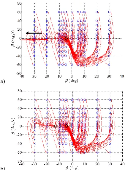
Fig. 3. Phase-plane plots for the controlled vehicle, at 80 km/h, with 50 deg of steering wheel angle. a) TV controller based only on the handling yaw rate; and b) TV controller with the sideslip-based yaw rate correction. *: points that diverge; ○: points that converge regardless of the sideslip-based correction; ×: points that converge to □; ◊: equilibrium of the vehicle in a);

□

:

3. SIMULATION RESULTS

A 𝛽̇(𝑡)-𝛽(𝑡) phase-plane analysis (where 𝑡 is time) is carried out with a vehicle simulation model including nonlinear tire behavior and the effect of the load transfers induced by the lateral acceleration. Several combinations of 𝛽 and 𝛽̇ are imposed as initial conditions for the vehicle simulator, which outputs the evolution of the model states in the time domain [23]. Then these can be represented in the 𝛽̇ -𝛽 plane, to identify the initial conditions from which the system response converges to an equilibrium.

Fig. 3 reports the simulation results for a high tire-road friction coefficient, at 80 km/h and with a constant 50 deg steering wheel angle (left turn), with two set-ups:

a) the vehicle with the TV controller using only the handling yaw rate, i.e., without sideslip-based correction (Fig. 3a)); and b) the vehicle with the TV controller including the sideslip-based correction of the reference yaw rate (Fig. 3b)). The handling yaw rate characteristics are those of the Sport Mode in [5].

Fig. 3a) shows that all the points characterized by an initial value of 𝛽 ≥ -10 deg converge to the equilibrium

𝛽𝑠𝑠= -4.5 deg, while for 𝛽 < -10 deg the system

diverges. The benefit of the sideslip-based correction is clearly visible in Fig. 3b), where the system converges regardless of the initial conditions. In particular, in this case there are two equilibria. In Fig. 3b) the originally stable points of Fig. 3a) converge to the same equilibrium as in Fig. 3a). On the other hand, the points originally unstable become stable, and they converge to a different equilibrium at approximately -15 deg, consistent with the values of 𝛽𝑎𝑐𝑡 and 𝛽𝑙𝑖𝑚 selected for the specific

simulations. In general, it was verified that the tuning parameters 𝛥𝑎𝑦, 𝐾𝑓 and 𝐾𝑠 affect the shape of the

trajectories, but not the location of the second sideslip angle equilibrium, which is mainly determined by 𝛽𝑙𝑖𝑚.

In summary, compared to the TV controller only based on the handling yaw rate [5], the proposed sideslip correction brings a significant extension of the stable region of vehicle operation in the 𝛽̇-𝛽 plane, even when the handling yaw rate is appropriate for the specific tire-road friction conditions. This positive result encouraged the experimental assessment of the controller formulation.

4. EXPERIMENTAL RESULTS

Experimental tests were conducted on the electric Range Rover Evoque prototype of the European Union funded project iCOMPOSE (Fig. 4). The vehicle includes four on-board electric drivetrains, each of them consisting of a switched reluctance electric motor drive, a single-speed transmission, and a half-shaft with constant velocity joints. The TV controller was implemented on a dSPACE AutoBox system installed on the vehicle.

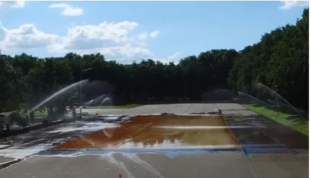
Fig. 4. The iCOMPOSE electric vehicle demonstrator with the Corrsys Datron sensor installed on the front end. The proving ground located in Weert (the Netherlands) was used for the experimental tests of this study (Fig. 5). The test area consists of a surface that is 150 m long and 41 m wide. The central part (50 m x 25 m) of such surface is characterized by a low friction area, made of epoxy and kept constantly wet by means of sprinklers. The remaining part of the proving ground is covered with common asphalt, which was dry during the tests. The friction coefficient in the low friction area is

study:

 The car is accelerated on a straight line until a reference speed value, 𝑉_𝑚, is steadily achieved.

 Once the vehicle is stabilized on 𝑉𝑚, a constant wheel

torque demand (100 Nm) is applied through the dSPACE system, thus bypassing the driver input on the accelerator pedal.

 The vehicle executes a slalom maneuver with cones located at 20 m from each other on a straight line.

 The vehicle starts the test on the high friction area, then enters the low friction area, and, at the end of the maneuver, goes back into the high friction area.

 𝑉𝑚 is defined as the maximum initial speed at which

the baseline vehicle (i.e., the vehicle without TV controller) can complete the maneuver without hitting any cone. The value of 𝑉_𝑚 was determined through multiple tests.

The test maneuver is particularly critical for stability control systems, because of the swift variation of the tire-road friction coefficient, which requires prompt adaptation of the controller. Hence, these test conditions are even more demanding than those typically achievable in a uniformly low-friction proving ground.

Fig. 5. The Weert proving ground (the Netherlands), with the central low friction area and sprinklers on each side.

The maneuver was executed with: i) the baseline vehicle, i.e., without TV controller; ii) the active vehicle with the TV controller only based on 𝑟ℎ , i.e., without

sideslip contribution in the definition of the reference yaw rate. The 𝑟ℎ look-up table was tuned for a high value

of the tire-road friction coefficient (dry tarmac); and iii) the active vehicle with the proposed SISO yaw rate and sideslip controller, and the same 𝑟ℎ set-up as in ii).

Configurations i), ii) and iii) are indicated respectively as B, YO and YS in the remainder.

Fig. 6 reports the time histories of the sideslip angle at the center of gravity and yaw rate for the three set-ups. In particular, the vehicle enters the low friction area at

≈4 s and leaves it at ≈9 s, with some variability caused by the difference in the velocity profiles of the multiple controller configurations along the maneuver. The results show that yaw rate-based TV control on its own can be dangerous if the friction conditions are not well estimated. In fact, the YO vehicle spins at ≈ 8.5 s, and is more aggressive than the B vehicle, with which the driver manages to complete the maneuver, despite the large peaks of sideslip angle. After 8.5 s, in the YO vehicle the sideslip angle has opposite sign with respect to the yaw

rate. The driver countersteers, but this is not sufficient to complete the test. The oversteer problem of the YO vehicle is caused by the excessively high absolute values of the reference (handling) yaw rate, designed for high friction conditions. The response of the YO vehicle is typical of a TV-controlled vehicle without a working friction estimator capable of modifying the reference yaw rate. The important conclusion is that a TV-controlled vehicle that is not properly tuned for low or variable friction conditions is potentially more dangerous than the corresponding baseline vehicle. The proposed sideslip-based correction of the reference yaw rate overcomes this issue. In fact, the YS vehicle adapts to the prevailing friction conditions and safely completes the maneuver, maintaining low values of sideslip angle.

a)

b)

Fig. 6. Experimental slalom maneuver. Time histories of: a) sideslip angle; and b) yaw rate, for the baseline vehicle (B), the vehicle with the TV controller only based on 𝑟ℎ

(YO), and the vehicle with the proposed SISO yaw rate and sideslip controller (YS).

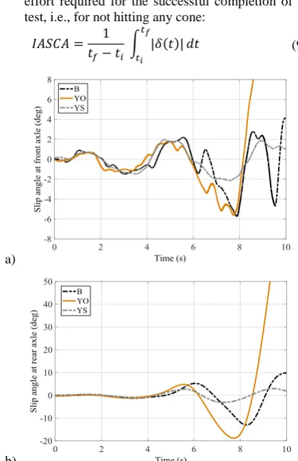
Fig. 7 reports the average slip angles of the front and rear axles. In particular, the front slip angle, 𝛼_𝐹𝐴, is calculated from the front sideslip angle and average steering angle of the two front wheels, 𝛿, i.e., 𝛼𝐹𝐴= 𝛿 −

𝛽𝐹𝐴. The rear slip angle, 𝛼𝑅𝐴, is equal in magnitude to

𝛽𝑅𝐴, i.e., 𝛼𝑅𝐴= −𝛽𝑅𝐴. From 0 s to 4 s, 𝛼𝐹𝐴 tends to be

larger in magnitude than 𝛼𝑅𝐴 for all cases, i.e., the

vehicle understeers. After 4 s, the B and YO vehicles present a rear slip angle significantly larger (in magnitude) than the front slip angle, i.e., they show an oversteering behavior, differently from the YS vehicle.

Five objective performance indicators are adopted for the assessment of each vehicle set-up:

 The root mean square value of the yaw rate error,

the feedback controller on yaw rate:

𝑅𝑀𝑆𝐸 = √ 1

𝑡𝑓− 𝑡𝑖∫ (𝑟𝑟𝑒𝑓(𝑡) − 𝑟(𝑡)) 2_𝑑𝑡 𝑡_𝑓

𝑡_𝑖

(6) where 𝑡_𝑖 and 𝑡_𝑓 represent the initial time and final time of the relevant part of the test, respectively. In particular, 𝑡𝑓− 𝑡𝑖 = 10 s for the specific tests.  The maximum absolute value of sideslip angle at the

rear axle, i.e., |𝛽𝑅𝐴,𝑚𝑎𝑥|. Based on the analysis

presented in Section 2, this corresponds to the maximum absolute value of the dynamic sideslip angle.

 The normalized integral of the absolute value of the control action, 𝐼𝐴𝐶𝐴, which evaluates the amount of direct yaw moment control effort:

𝐼𝐴𝐶𝐴 = 1

𝑡𝑓− 𝑡𝑖 ∫ |𝑀𝑧(𝑡)| 𝑡𝑓

𝑡_𝑖

𝑑𝑡 (7)

 ∆𝑉%, which provides the magnitude of the vehicle speed reduction during the test, expressed as a percentage of the initial speed, 𝑉𝑚:

∆𝑉% = 100𝑉𝑚− 𝑉(𝑡𝑓)

𝑉𝑚 (8)

 The normalized integral of the absolute value of the steering wheel control action applied by the driver,

𝐼𝐴𝑆𝐶𝐴. This indicator represents the steering wheel effort required for the successful completion of the test, i.e., for not hitting any cone:

𝐼𝐴𝑆𝐶𝐴 = 1

𝑡𝑓− 𝑡𝑖 ∫ |𝛿(𝑡)| 𝑡_𝑓

𝑡_𝑖 𝑑𝑡 (9)

a)

b)

Fig. 7. Experimental slalom maneuver. Time histories of: a) 𝛼𝐹𝐴(𝑡) ; and b) 𝛼𝑅𝐴(𝑡) = −𝛽𝑅𝐴(𝑡) , for the three

vehicle set-ups.

Based on Table 1 and Fig. 6, the B vehicle has a very limited yaw rate tracking performance, simply because there is no yaw rate control. The maximum value of sideslip angle is significantly higher than a safety-critical acceptable value (approximately 4-5 deg); nevertheless, the driver was able to complete the maneuver. The YO vehicle is characterized by a large control effort; yet it is not able to follow the reference yaw rate (high 𝑅𝑀𝑆𝐸), as it spins due to the high friction conditions assumed by the controller without sideslip-based correction. For the same reason, the steering effort and the reduction in vehicle speed are significant for the YO vehicle, worse than for the B vehicle. On the other hand, the YS vehicle guarantees the smallest |𝛽𝑅𝐴,𝑚𝑎𝑥|, the best yaw rate

tracking performance, the smallest vehicle speed reduction, and the lowest steering effort for the driver. Hence, the safety benefit achieved with the proposed controller is evident.

Table 1. Performance indicators for the experimental maneuver, 𝑉𝑚= 37 km/h.

Vehicle layout

𝑅𝑀𝑆𝐸

(deg/s)

|𝛽𝑅𝐴,𝑚𝑎𝑥|

(deg)

𝐼𝐴𝐶𝐴

(Nm) ∆V%

𝐼𝐴𝑆𝐶𝐴

(deg) B 17.9 13.0 0 21.3 54.4 YO 47.1 85.6 1224 56.1 87.8 YS 3.4 3.1 1013 5.2 29.0

5. CONCLUSION

The paper demonstrated that effective yaw rate control with appropriate constraints on sideslip angle is achievable with a SISO control formulation, i.e., with a simple yaw rate controller, in which the reference yaw rate is modified according to the measured or estimated sideslip angle. The proposed controller uses the sideslip angle at the rear axle, 𝛽𝑅𝐴, as control variable, because it

causes the sideslip-based intervention only when it is actually needed, i.e., when there is a significant dynamic sideslip angle. On the other hand, the adoption of the sideslip angle at the center of gravity or the front axle would imply interventions of the sideslip correction in conditions of large steering wheel inputs and trajectory curvatures. These correspond to large kinematic sideslip angle values, which do not necessarily result into safety-critical vehicle operation.

The simulation results show that the proposed controller significantly extends the stable region of vehicle operation on the 𝛽̇-𝛽 phase-plane for high values of the tire-road friction coefficient. This means that sideslip control is beneficial also when the handling yaw rate is appropriately designed for the available friction level.

the vehicle with the TV controller with a reference yaw rate for high friction conditions. Based on the experiments, in variable friction conditions it is more important to have appropriate and swiftly adaptable generation of the reference yaw rate signal, rather than an advanced control structure focused on providing excellent tracking performance.

ACKNOWLEDGEMENTS

The research leading to these results has received funding from the European Union Seventh Framework Programme FP7/2007-2013 under Grant Agreement No. 608897 (iCOMPOSE project).

REFERENCES

[1] Esmailzadeh, E., Goodarzi, A., Vossoughi, G.R., "Optimal yaw moment control law for improved vehicle handling," Mechatronics, 13(7), pp. 659-675, 2003.

[2] Kaiser, G., "Torque vectoring - linear parameter-varying control for an electric vehicle," PhD Thesis, Hamburg-Harburg Technical University, 2014. [3] Tota, A., Lenzo, B., Lu, Q., Sorniotti, A., Gruber, P.,

Fallah, S., Velardocchia, M., Galvagno, E., De Smet, J., "On the experimental analysis of integral sliding modes for yaw rate and sideslip control," International Journal of Automotive Technology, 2018 (in press).

[4] Wang, Z., Montanaro, U., Fallah, S., Sorniotti, A., Lenzo, B., "A gain scheduled robust linear quadratic regulator for vehicle direct yaw moment control," Mechatronics, 51, pp. 31-45, 2018.

[5] De Novellis, L., Sorniotti, A., Gruber, P., "Driving modes for designing the cornering response of fully electric vehicles with multiple motors," Mechanical Systems and Signal Processing, 64-65, pp. 1-15, 2015.

[6] De Novellis, L., Sorniotti, A., Gruber, P., Pennycott, A, "Comparison of feedback control techniques for torque-vectoring control of fully electric vehicles," IEEE Transactions on Vehicular Technology, 63(8), pp. 3612-3623, 2014.

[7] Lenzo, B., Sorniotti, A., De Filippis, G., Gruber, P., Sannen, K., "Understeer characteristics for energy-efficient fully electric vehicles with multiple motors," International Battery, Hybrid and Fuel Cell Electric Vehicle Symposium (EVS29), 2016. [8] Bucchi, F., Lenzo, B., Frendo, F., Sorniotti, A., De

Nijs, W., "The effect of the front-to-rear wheel torque distribution on vehicle handling: an experimental assessment," 25th _{International}

Symposium on dynamics of vehicles on roads and tracks (IAVSD), 2017.

[9] Bucchi, F., Frendo, F., "A new formulation of the understeer coefficient to relate yaw torque and vehicle handling," Vehicle System Dynamics, 54(6), pp. 831-847, 2016.

[10] Liu, C.S., Peng, H., "Road friction coefficient estimation for vehicle path prediction," Vehicle system dynamics, 25(S1), pp. 413-425, 1996. [11] Voser, C., Hindiyeh, R., Gerdes, J., "Analysis and

control of high sideslip manoeuvres," Vehicle System Dynamics, 48(S1), pp. 317-336, 2010. [12] Lenzo, B., Sorniotti, A., Gruber, P., Sannen, K., "On

the experimental analysis of single input single output control of yaw rate and sideslip angle," International Journal of Automotive Technology, 18(5), pp. 799-811, 2017.

[13] Lu, Q., Gentile, P., Tota, A., Sorniotti, A., Gruber, P., Costamagna, F., De Smet, J., "Enhancing vehicle cornering limit through sideslip and yaw rate control," Mechanical Systems and Signal Processing, 75, pp. 455-472, 2016.

[14] Lenzo, B., De Filippis, G., Dizqah, A.M., Sorniotti, A., Gruber, P., Fallah, S., De Nijs, W., "Torque distribution strategies for energy-efficient electric vehicles with multiple drivetrains," Journal of Dynamic Systems, Measurement, and Control, 139(12), p. 121004, 2017.

[15] De Filippis, G., Lenzo, B., Sorniotti, A., Gruber, P., De Nijs, W., "Energy-efficient torque-vectoring control of electric vehicles with multiple drivetrains," IEEE Transactions on Vehicular Technology, 2018 (in press).

[16] Teng, G.W., Xiong, L., Leng, B., Hu, S.L., "A novel reference model for vehicle dynamics control," 24th

International Symposium on Dynamics of Vehicles on Roads and Tracks (IAVSD), 2015.

[17] Guiggiani, M., "The science of vehicle dynamics: handling, braking, and ride of road and race cars," Springer, 2014.

[18] Genta, G., "Motor vehicle dynamics: modeling and simulation," World Scientific, 1997.

[19] Chindamo, D., Lenzo, B., Gadola, M. "On the vehicle sideslip angle estimation: a literature review of methods, models, and innovations," Applied Sciences, 8(3), p. 355, 2018.

[20] Farroni, F., Pasquino, N., Rocca, E., Timpone, F., "A comparison among different methods to estimate vehicle sideslip angle," World Congress on Engineering, 2015.

[21] Gadola, M., Chindamo, D., Romano, M., Padula, F., "Development and validation of a Kalman filter-based model for vehicle slip angle estimation," Vehicle System Dynamics, 52(1), pp. 68-84, 2014. [22] Baffet, G., Charara, A., Stephant, J., "Sideslip angle,

lateral tire force and road friction estimation in simulations and experiments," IEEE International Conference on Control Applications, 2006. [23] Farroni, F., Russo, M., Russo, R., Terzo, M.,