Design of a Sliding Mode Controller (SMC) based on Reaching Law

Design of a Sliding Mode Controller (SMC) based on

Reaching Law

Abhishek Chaudhary

Control & Instrumentation, EED,

Delhi Technological University (DTU),

Delhi – 110042, India

Bharat Bhushan

Electrical Engineering Dept. (EED)

Delhi Technological University (DTU),

Delhi – 110042, India

ABSTRACT

This paper presents a principle for the design of a sliding mode controller. Sliding Mode is based on Reaching law includes reaching phase and sliding phase. This controller can be implemented on a nonlinear plant to make it work as a slightly linear plant. This is done by using implementing the equations of controller into the Simulink model to obtain the controlled output.

Keywords

Sliding mode controller, MATLAB, Simulink, MATLAB coding.

1.

INTRODUCTION

Interests in the sliding mode controller is being increased now a days among the researchers in control system engineering. These controller are being implemented on to the non-linear systems in order to make them work like a linear systems for a slight duration of consideration. SMC are used for underactuated systems basically [1],[2].

Control researchers have given considerable attention to many examples of control problems associated with underactuated mechanical systems and different control strategies have been proposed. Use of decoupling algorithm to design the different controllers for underactuated systems has given satisfied results in researches. [2]

The variety of application of SMC controllers is very wide due to its robustness, associated to disturbance rejection capacity and simplicity [3]. SMC is a robust method for the systems which possesses some non-linearity owing to dynamic response and is being used in converters for many years [4]. SMC based controller technique is applied to buck boost and Cuk converter circuits in [5, 6, 7].

In [8], a sliding mode controller is combined to a Kalman filter in a three phase unity power factor rectifier. On the other hand, the discrete time sliding mode approach is very attractive due to the possibility of easy implementation in digital controllers, and this approach has been developed by several researchers [9],[10],[11]. In literature, some authors have reported the use of higher order sliding mode controllers for different machines [12],[13],[14],[15],[16],[17]. While most of this work used SMC as an observer [12],[13],[14], the authors in [15],[16],[17] used SMC as a controller.

In this paper, the approach to implement a SMC controller on a plant is provided. The results of the controller on the plant is obtained on the MATLAB platform. The coding and the simulation, both the techniques are used for obtaining these results and the same is shown in this paper. It is compulsory for the sliding mode controller to satisfy the Lyapunov equation i.e. Lyapunov function and the matrix used in this process must satisfy the Hurwitz matrix else we will never get the stable results. Section II is giving the general design of a

SMC controller and then Section III is adding the reaching law to the general model of SMC controller. The equations obtained in these two sections are put into an example in section III to obtain the required of sliding mode controller based on reaching law.

Sliding Mode controllers are well known for their robustness and stability. The nature of the controller is to ideally operate at an infinite switching frequency such that the controlled variable scan track a certain reference path to achieve the desired dynamic response and steady-state operation [18]. This requirement for operation at infinite switching frequency, however, challenges the feasibility of applying SM controllers in power converters. This is because extreme high speed switching in power converters results in excessive switching losses, inductor and transformer core losses, and electromagnetic interference (EMI) noise issues [19]. Hence, for SM controllers to be applicable to power converters, their switching frequencies must be constricted within a practical range. Nevertheless, this constriction of the SM controller’s switching frequency transforms the controller into a type of quasi-sliding-mode (QSM) controller, which operates as an approximation of the ideal SM controller. The consequence of this transformation is the reduction of the system’s robustness. Clearly, the proximity of QSM to the ideal SM controller will be closer as switching frequency tends toward infinity. Since all SM controllers in practical power converters are frequency-limited, they are, strictly speaking, QSM controllers. For brevity and consistency with previous publications, the term SM controller will be used in the sequel.

46 circumstance, it is meaningful to design sliding-mode

controllers based on output information alone, and many works have explored the development of sliding-mode output feedback control, which can be seen in [28] and [29] and the references therein. Among the existing output feedback control approaches, the static output feedback control appears to be the simplest and cheapest approach. Some examples of investigation on static output feedback SMC strategies can be found in [30]–[32].

2.

DESIGN OF SMC

Consider a plant as:

𝐽𝜃 𝑡 = 𝑢 𝑡 + 𝑑(𝑡) (1)

Where,

J → moment of inertia

𝜃 𝑡 → Angle signal

𝑢 𝑡 → Control input

𝑑(𝑡 ) → Disturbance

Design the sliding mode function as:

𝑠 𝑡 = 𝑐𝑒 𝑡 + 𝑒 (𝑡) (2)

Where c must satisfies Hurwitz condition, c>0

Tracking error and its derivative value is

𝑒 𝑡 = 𝜃 𝑡 − 𝜃𝑑(𝑡),

𝑒 𝑡 = 𝜃 𝑡 − 𝜃𝑑 (𝑡)

Where, 𝜃𝑑 (𝑡)is the ideal position signal.

To satisfy the conditions of sliding mode controller, we must satisfy the position tracking error and speed tracking error tends to zero as time reaches to ∞. While doing so we must put s(t)=0.

From eq. (2):

𝑠 𝑡 = 𝑐𝑒 𝑡 + 𝑒 𝑡

Which give → 𝑠 𝑡 = 𝑐𝑒 𝑡 + 𝑒 (𝑡)

= 𝑐𝑒 𝑡 + 𝜃 𝑡 − 𝜃𝑑 𝑡

= 𝑐𝑒 𝑡 + 1

𝐽(𝑢 𝑡 + 𝑑(𝑡)) − 𝜃𝑑 𝑡 (3) The we have:

𝑠𝑠 = 𝑠(𝑐𝑒 𝑡 + 1

𝐽(𝑢 𝑡 + 𝑑(𝑡)) − 𝜃𝑑 𝑡 )

To guarantee 𝑠𝑠 < 0, design the sliding mode controller as:

𝑢 𝑡 = 𝐽(-𝑐𝑒 𝑡 + 𝜃𝑑 𝑡 − 1

𝐽(𝑘𝑠 + 𝑁𝑠𝑔𝑛𝑠) (4) Design the Lyapunov function as:

V=1 2𝑠

2

We obtain:

𝑉 = 𝑠𝑠 =s(−𝑘𝑠 −1

𝐽𝑁𝑠𝑔𝑛𝑠 + 1 𝐽𝑑(𝑡))

=1 𝐽(−𝑘𝑠

2_{− 𝑁 𝑠 + 𝑠𝑑(𝑡)}

<=1 𝐽𝑘𝑠

2

Then we have:

𝑉 < =1 𝐽

𝑘𝑠2

Hence, if we put k as positive constant value then V (t) will tend to zero exponentially with k value and sliding mode controller will be formed.

3.

SMC MODEL ON REACHING LAW

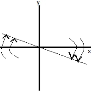
Sliding mode controller based on reaching law include reaching phase and sliding phase. The reaching phase drive system to stable manifold, the sliding phase drive system slide to equilibrium. Figure 1.1 is showing the idea of sliding mode using the reaching law more clearly.

Figure 1.1 The Idea of Sliding Mode Control using reaching law

Consider the plant as:

𝑥 𝑡 = 𝑓 𝑥, 𝑡 + 𝑏𝑢 𝑡 + 𝑑(𝑡) (5)

Where, 𝑓 𝑥, 𝑡 & 𝑏are known parameters and d(t) is the unknown disturbance:

Design the sliding mode function as:

𝑠 𝑡 = 𝑐𝑒 𝑡 + 𝑒 (𝑡) (6)

c is satisfying Hurwitz.

Tracking error and derivative value is:

e = 𝑥𝑑− 𝑥1

𝑒 = 𝑥𝑑 − 𝑥1

Where, 𝑥1= 𝑥 𝑎𝑛𝑑 𝑥𝑑is the ideal position:

Then we have,

𝑠 𝑡 = 𝑐𝑒 𝑡 + 𝑒 (𝑡)

𝑠 𝑡 = 𝑐 𝑥𝑑 − 𝑥1 + (𝑥𝑑 − 𝑥 )

From eq. (5):

𝑠 𝑡 = 𝑐 𝑥𝑑 − 𝑥1 + (𝑥𝑑 − 𝑓 − 𝑏𝑢 − 𝑑) (7)

Adopting the condition of exponential reaching law, we have:

𝑠 𝑡 = −𝑁𝑠𝑔𝑛𝑠 − 𝑘𝑠 (8)

Where, -ks is an exponential term with s= s(0)𝑒−𝑘𝑡_{and –} Nsgns is a constant term.

𝑐 𝑥𝑑 − 𝑥1 + 𝑥𝑑 − 𝑓 − 𝑏𝑢 − 𝑑 = −𝑁𝑠𝑔𝑛𝑠 − 𝑘𝑠 (9)

From eq. (5) & (9), SMC may be designed as:

𝑢 𝑡 =1

𝑏(𝑐 𝑥𝑑 − 𝑥1 + 𝑥𝑑 − 𝑓 − 𝑏𝑢 − 𝑑 + 𝑁𝑠𝑔𝑛𝑠 + 𝑘𝑠)

(10)

All the quantities in this equation except for d(t) are known.

Now putting eq. (10) in eq. (7) we get:

𝑠 𝑡 = −𝑁𝑠𝑔𝑛𝑠 − 𝑘𝑠 − 𝐷𝑠𝑔𝑛𝑠 (11)

Where, D is the overall disturbance. Then:

𝑠𝑠 𝑡 = 𝑠(−𝑁𝑠𝑔𝑛𝑠 − 𝑘𝑠 − 𝐷𝑠𝑔𝑛𝑠)

= −𝑘𝑠2_{− 𝑁 𝑠 − 𝐷 𝑠 (12)}

Using the Lyapunov function from section II of this paper:

V=1 2𝑠

2

Then we get:

𝑉 = 𝑠𝑠 𝑡 = −𝑘𝑠2_{− 𝑁 𝑠 − 𝐷 𝑠}

Which definitely gives:

𝑉 𝑡 ≤ 𝑒−2𝑘𝑡_{𝑉 0 . (13)}

And hence, we can see that the sliding mode function 𝑠(𝑡)

will tends to zero exponentially with k value.

4.

SIMULATION EXAMPLE

Consider the plant as:

𝑥 𝑡 = 𝑓 𝑥, 𝑡 + 𝑏𝑢 𝑡 + 𝑑(𝑡) (5)

With following parametric values:

f = -25𝑥 ,

b = 133

Initial states as [-0.15 0.15]

c=15

N=0.5

k=10.

D=10.1

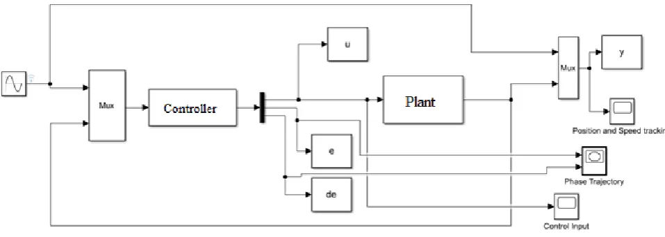
These values are put into the given system and in the required equations of the section II and section III of this paper. Then by using the MATLAB coding skills two different .m files are made up into the MATLAB platform. One is for the controller and other .m file is for the plant.

Both the files then transcribed into the SIMULATION block of the MATLAB platform.

In Fig. 1.2 the same simulation block is shown. The Controller and Plant block shown here are inscribed with MATLAB coding / programming of SMC controller’s equations and TORA system’s equations respectively.

Figure 1.2 Block Diagram of Simulation Model used

As we can see easily in the block diagram, 3 different output plots are shown.

48

Fig.2 Phase Trajectory of the Sliding Mode Controller

Figure 3 is all about the tracking of speed and position of the controller parameters. As we can see in the block diagram, the output of the plant is sent to the Mux for the comparison and the output purposes. There the tracking of speed and position is made possible.

Fig.3 Position and Speed Tracking

Figure 4 is showing the controlled input of the plant which is actually the ouput of the controller. This control input is showing the reaching range of the contoller parameter. In this figure the reaching law is actually verified by the SMC controller.

Fig.4 Control Input to the plant

5.

CONCLUSION

After observing the results, we are quite clear about the fact that the gain k plays an important part in the stability and working of a controller. The figures are showing the results of the SMC on the given plant and also verifying the reaching law condition as the controller is implemented on the given system within the reaching phase and the sliding phase. These implementations are done with the help of mathematical calculations shown in second and third sections of this paper. Hence, the implementation of Sliding Mode Controller using reaching law on a plant is verified.

6.

REFERENCES

[1] H. Ashrafiuona, R.S. Erwinb, “Sliding Mode Control Of Underactuated Multibody Systems And Its Application To Shape Change Control”, Int. J. Control. 81 (12) (2008) 1849-1858.

[2] Rong Xu, Umit Ozguner, “Sliding Mode Control Of A Class Of Underactuated Systems”, Automatica 44(2008) 233-248.

[3] V. Utkin, J. Guldner, S. Jingxin, “Sliding Mode Control In Electromechanical Systems”. Vol 34. Crc Press, 2009.

[4] R. Venkataramanan, “Sliding Mode Control Of Power Converters” Phd. Diss., California Institute Of Technology, 1986.

[5] F. Ahmad, A. Rasool, E.E. Ozosoy, A. Sabanovic, M. Elitas, “Design Of A Robust Cascaded Controller For Cuk Converters” IEEE International Power Electronics And Motion Control Conf. (Pemc), Pp. 80-85, 2016.

[6] S.C. Tan, Y.M. Lai, C.K. Tse, M.K. Cheung, “A Fixed-Frequency Pulse Width Modulation Based Quasi-Sliding-Mode- Controller For Buck Converters”, IEEE Trans. On Power Elect. Vol. 20, No. 3 Pp. 1379-1392, Nov. 2005.

[7] K.K. Leung, H.S. Chung, “Dynamic Hysteresis Band Control Of The Buck Converter With Fast Transient Response, IEEE Trans.On Circuits And Systems Ii: Express Briefs, Vol.52, No. 7, Pp.398-402, July 2005.

Switching Frequency”, IEEE Trans. Power Electron., Vol.31, No. 1, Pp. 758-769, Jan. 2016.

[9] W. Gao, Y. Wang, And A. Homaifa, “Discrete Time Variable Structure Control Systems”, IEEE Trans. Ind. Electron., Vol. 42 No. 2, Pp 117-122, Apr. 1995.

[10]A. Bartoszewicz, “Discrete Time Quasi Sliding Mode Control Strategies”, IEEE Trans Ind. Electron., Vol. 45, No. 4, Pp. 633-637, Aug. 1998.

[11]J. Zhang, G. Feng, Y. Xia. “Design Of Estimator-Based Sliding-Mode-Output Feedback Controller For Discrete Time Systems”, IEEE Trans. Ind. Electron., Vol. 61, No. 5, Pp. 2432-2440, May 2014.

[12]L. Zhao, J. Huang, H. Liu, B. Li, W. Kong, “Second Order Sliding Mode Observer With Online Parameter Indentification For Sensorless Induction Motor Drives”, IEEE Trans. Ind. Electron., Vol. 61, No. 10, Pp. 5280-5289, Oct. 2014.

[13]S. Di Gennaro, J. Rivera Dominguez, M. Meza, “Sensorless High Order Sliding Mode Control Of Induction Motors With Core Loss”, IEEE Trans. Ind. Electron., Vol. 61, Pp. 2678-2689, Jun. 2014.

[14]M.T. Angulo And R. V. Carrillo Serrano, “Estimating Rotor Parameters In Induction Motors Using High Order Sliding Mode Algorithms”, Iet Control Theory Appl., Vol. 9, No. 4, Pp. 573-578, 2015.

[15]D. Traore, F. Plestan, A. Glumineau, J. De Leon, “Sensorless Induction Motor: High Order Sliding Mode Controller And Adaptive Interconnected Observer”, IEEE Trans. Ind. Electron., Vol. 55, No. 11, Pp. 3818-3827, Nov. 2008.

[16]M. Rashed , K.B. Goh, M.W. Dunnigan, P.F. A. Macconnel, A.F. Stronach, B.W. Williams, “Sensorless Second Order Sliding Mode Speed Control Of A Voltage Fed Induction Motor Drive Using Nonlinear State Feedback”, Iee Proc. On Elect. Pow. Appl., Vol. 152, No. 5, Pp. 1127-1136, Sept. 2005.

[17]A. Pisano, A. Davila, L. Fridman, E. Usai, “Cascade Control Of Pm Dc Drives Via Second Order Sliding Mode Technique”, IEEE Trans. Ind. Electron., Vol. 55, No. 11, Pp. 3846-3854, Nov. 2008.

[18]V. Utkin, J. Guldner, and J. X. Shi, Sliding Mode Control in Electromechanical Systems. London, UK: Taylor and Francis, 1999.

[19]H.W.Whittington,B.W.Flynn,

andD.E.Macpherson,Switched Mode Power Supplies: Design and Construction, 2nd ed. New York: Wiley, 1997

[20]W. Gao, Y. Wang, and A. Homaifa, “Discrete-time variable structure control systems,” IEEE Trans. Ind. Electron., vol. 42, no. 2, pp. 117–122, Apr. 1995.

[21]A. Bartoszewicz, “Discrete-time quasi-sliding-mode control strategies,” IEEE Trans. Ind. Electron., vol. 45, no. 4, pp. 633–637, Aug. 1998.

[22]J. Hu, Z. Wang, H. Gao, and L. K. Stergioulas, “Robust sliding mode control for discrete stochastic systems with mixed time delays, randomly occurring uncertainties, and randomly occurring nonlinearities,” IEEE Trans. Ind. Electron., vol. 59, no. 7, pp. 3008–3015, Jul. 2012.

[23]Y. Xia, G. Liu, P. Shi, J. Chen, D. Rees, and J. Liang, “Sliding mode control of uncertain linear discrete time systems with input delay,” IET Control Theory Appl., vol. 1, no. 4, pp. 1169–1175, Jul. 2007.

[24]Y. Niu, D. W. C. Ho, and Z. Wang, “Improved sliding

mode control for

discrete-timesystemsviareachinglaw,”IETControlTheoryAppl.,vol .4, no. 11, pp. 2245–2251, Nov. 2010.

[25]Y. Xia, M. Fu, P. Shi, and M. Wang, “Robust sliding mode control for uncertain discrete-time systems with time delay,” IET Control Theory Appl., vol. 4, no. 4, pp. 613–624, Apr. 2010.

[26]J.Zhang,J.Lam,andY.Xia,“Outputfeedbackslidingmodeco ntrolunder networked environment,” Int. J. Syst. Sci., vol. 44, no. 4, pp. 750–759, Apr. 2013.

[27]Y.NiuandD.W.C.Ho,“Designofslidingmodecontrolsubjec ttopacket losses,” IEEE Trans. Autom. Control, vol. 55, no. 11, pp. 2623–2628, Nov. 2010.

[28]C. Edwards and S. K. Spurgeon, Sliding Mode Control: Theory and Applications. New York, NY, USA: Taylor and Francis, 1998.

[29]H. H. Choi, “Sliding-mode output feedback control design,” IEEE Trans. Ind. Electron., vol. 55, no. 11, pp. 4047–4054, Nov. 2008.

[30]A. Seuret, C. Edwards, S. K. Spurgeon, and E. Fridman, “Static output feedback sliding mode control design via an artificial stabilizing delay,” IEEE Trans. Autom. Control, vol. 54, no. 2, pp. 256–265, Feb. 2009.

[31]J. Zhang, P. Shi, and Y. Xia, “Robust adaptive sliding mode control for fuzzy systems with mismatched uncertainties,” IEEE Trans. Fuzzy Syst., vol. 18, no. 4, pp. 700–711, Aug. 2010.