Testing independence for multivariate time series via the auto distance correlation matrix

auto-distance correlation matrix

Konstantinos Fokianos

Maria Pitsillou

Department of Mathematics & Statistics, University of Cyprus

e-mail: {fokianos, pitsillou.maria}@ucy.ac.cy

Submitted for publication: April 2016

First Revision: June 2017

Second Revision: November 2017

Abstract

We introduce the matrix multivariate auto-distance covariance and correlation functions for time series, dis-cuss their interpretation and develop consistent estimators for practical implementation. We also develop a test for testing the independent and identically distributed hypothesis for multivariate time series data and show that it performs better than the multivariate Ljung–Box test. We discuss computational aspects and present a data example to illustrate the methodology.

1

Introduction

In applications from fields such as economics (e.g. Tsay, 2014), medicine (McLachlan et al., 2004) or

environ-metrics (Hipel and McLeod, 1994) we observe several time series evolving simultaneously. Analyzing each

com-ponent separately might lead to wrong conclusions because of possible interrelationships among the series. Such

relationships are usually identified by employing the autocovariance function. For ad-dimensional stationary time

series{Xt, t∈Z}with meanµ, the autocovariance function is defined by

Γ(j) = En(Xt+j−µ)(Xt−µ)| o

=nγrm(j) od

r,m=1 (j∈Z).

A consistent estimator is the sample autocorrelation function (Brockwell and Davis, 1991, p. 397)

ˆ Γ(j) =

     

    

n−1

n−j X

t=1

(Xt+j−X¯)(Xt−X¯)|, 0≤j≤n−1,

n−1

n X

t=−j+1

(Xt+j−X¯)(Xt−X¯)|, −n+ 1≤j <0,

which is often used to measure pairwise dependence. The multivariate Ljung–Box test statistic (Hosking, 1980; Li

and McLeod, 1981) is formed in terms as

mLB=n2

p X

j=1

(n−j)−1trnΓˆ|(j)ˆΓ−1(0)ˆΓ(j)ˆΓ−1(0)o, (1) and it is widely applied for testing the hypothesesΓ(1) =· · · = Γ(p) = 0. However, application of (1) should

be done carefully because the number of lags included is held constant but, in practice, the dependence might

be of higher order (Hong, 1998, 2000; Xiao and Wu, 2014). Furthermore, the autocovariance function cannot

always detect serial dependence for purely non-Gaussian and non-linear models, though it is suitable for Gaussian

models. Test statistics which are based on the autocovariance function for testing independence are not consistent

against alternatives for models with zero autocovariance (Romano and Thombs, 1996; Shao, 2011), so alternative

dependence measures should be studied (Tjøstheim, 1996; Lacal and Tjøstheim, 2017, 2018).

We study the auto-distance covariance function as a suitable statistic for detecting nonlinear relationships in

gave an early treatment and Zhou (2012), Dueck et al. (2014), Fokianos and Pitsillou (2017) and Davis et al. (2016)

extended it to time series. Work on the closely related notion of the Hilbert–Schmidt independence criterion

in-cludes Sejdinovic et al. (2013) and Gretton et al. (2008). In the present paper, we introduce the auto-distance

covariance matrix to identify possible non-linear relationships among the components of a vector series {Xt}

and show that its sample version is a consistent estimator of the population auto-distance covariance matrix. The

sample auto-distance covariance matrix may be used to construct tests for independence of multivariate time

se-ries. This is accomplished by following Hong (1999), who introduced the so-called generalized spectral density

function. The generalized spectral density matrix captures all the forms of dependence because it is constructed

by using the characteristic function. Hence, we can develop statistics for testing independence by considering an

increasing number of lags.

The present paper extends Zhou (2012) and Fokianos and Pitsillou (2017), who consider univariate testing of

inde-pendence based on auto-distance covariance and Székely et al. (2007), since some of our results can be transferred

to independent data. Indeed, using the auto-distance covariance matrix for identification of possible dependencies

among the components of a random vector could give rise to novel dimension-reduction methods. All methods are

available in the R packagedCovTS(Pitsillou and Fokianos, 2016).

2

Auto-Distance Covariance Matrix

2.1

Definitions

Suppose that{Xt, t∈Z}is ad-variate strictly stationary time series. Denote its cumulative distribution function byF(x1, . . . , xd)and assume thatE(|Xt;r|) <∞, forr= 1, . . . , d. LetFr(·)denote the marginal distribution

function of{Xt;r}andFrm(·,·)that of(Xt;r, Xt;m)withr, m= 1, . . . , d. Let{Xt:t= 1, . . . , n}be a sample

of sizen. Zhou (2012), by extending the results of Székely et al. (2007), defines the distance covariance function

for multivariate time series, but without taking into account possible cross-dependencies between all possible

between the joint characteristic function and the marginal characteristic functions of the pair(Xt;r, Xt+j;m), for

r, m= 1, . . . , d. Denote the joint characteristic function ofXt;randXt+j;mby

φ(_jr,m)(u, v) =E

"

expni(uXt;r+vXt+j;m) o

#

(u, v∈R;j∈Z),

wherer, m = 1, . . . , d andi2 _{= −1. Letφ}(r)_{(u) = E}h_expn_i(uX

t;r) oi

denote the marginal characteristic

function ofXt;rforr= 1, . . . , d. Let

Σj(u, v) = n

σ_j(r,m)(u, v)o (j∈Z) (2)

denote thed×dmatrix whose(r, m)element is

σ(_jr,m)(u, v) = covnexp(iuXt;r),exp(ivXt+j;m) o

=φ(_jr,m)(u, v)−φ(r)(u)φ(m)(v). (3) Ifσ(_jr,m)(u, v) = 0for all(u, v)∈R2then the random variablesXt;randXt+j;mare independent for allj. Let

thek · kW-norm ofσj(r,m)(u, v)be defined by kσ_j(r,m)(u, v)k2_W =

Z

R2 σ

(r,m)

j (u, v)

2

W(du, dv) (j∈Z),

whereW(·,·)is an arbitrary positive weight function such thatkσ(_jr,m)(u, v)k2

W <∞. Feuerverger (1993) and

Székely et al. (2007) employ a non-integrable weight function,

W(du, dv) = 1

π|u|2

1

π|v|2dudv. (4)

The choice ofW(·,·)is key in this work. Obviously, (A.4) is non-integrable inR2, but, choices withRdW<∞ are possible. Following Hong (1999) and Chen and Hong (2012), suppose thatW(·,·) :_R2_→

R+is nondecreas-ing with bounded total variation. This obviously holds forW(du, dv) =dΦ(u)dΦ(v), whereΦ(·)is the standard

normal cumulative distribution function. In this case,kσ(_jr,m)(u, v)k2

Wcan be computed by Monte Carlo

simula-tion. For related work, see also Meintanis and Iliopoulos (2008) and Hlávka et al. (2011). In what follows we use

(A.4) throughout, taking into account the fact that integrable weight functions might miss potential dependence

Definition 1The pairwise auto-distance covariance function betweenXt;randXt+j;mis denoted byVrm(j)and

defined as the positive square root of

V_rm2 (j) = kσ_j(r,m)(u, v)k2

W (r, m= 1, . . . , d; j ∈Z), (5)

withW(·,·)given by(A.4). The auto-distance covariance matrix of{Xt}at lagjwill be denoted byV(j)and is

thed×dmatrix

V(j) =

(

Vrm(j) )d

r,m=1

(j ∈Z). (6)

Clearly,V2

rm(j)≥0, for alljandXt;randXt+j;mare independent if and only ifVrm2 (j) = 0. Furthermore, we

define thed×dmatrices

V(2)(j) =

(

V_rm2 (j)

)d

r,m=1

(j∈_Z). (7)

Definition 1 is valid for any weight functionW(·,·)such thatVrm2 (j) < ∞; with (A.4), it is a pairwise

auto-distance covariance function.

Definition 2The pairwise auto-distance correlation function betweenXt;randXt+j;mis denoted byRrm(j)and

defined as the positive square root of

R2rm(j) =

Vrm2 (j) n

V2

rr(0)Vmm2 (0)

o1/2 (r, m= 1, . . . , d; j∈Z),

provided thatVrr(0)Vmm(0)= 06 . The auto-distance correlation matrix of{Xt}at lagjis

R(j) =

(

Rrm(j) )d

r,m=1

(j∈Z).

Similarly, define thed×dmatrices

R(2)(j) =

(

R2_rm(j)

)d

r,m=1

(j∈_Z).

Then (7) shows thatR(2)_{(j) =D}−1_V(2)_(j)D−1_{, whereD =diag}

Vrr(0)

, (r= 1, . . . , d). All above

popula-tion quantities exist and are well-defined because of standard properties of the characteristic funcpopula-tion. Davis et al.

Whenj6= 0,Vrm(j)measures the dependence ofXt;ronXt+j;m. Forj >0and ifVrm(j)>0, we say that the

seriesXt;mleads the seriesXt;rat lagj. In general,Vrm(j)6=Vmr(j)forr6=m, since they measure different

types of dependence between the series{Xt;r} and{Xt;m}for allr, m = 1, . . . , d. Thus,V(j)andR(j)are

non-symmetric matrices, but by stationarity,

Vrm2 (−j) = kcov n

exp(iuXt;r),exp(ivXt−j;m) o

k2

W

= kcovnexp(iuXt;m),exp(ivXt+j;r) o

k2_W =V_mr2 (j), r, m= 1, . . . , d.

Consequently,V(−j) =V|_{(j)andR(−j) =R}|_{(j), because the matricesV(j)andR(j)have as elements the}

positive square roots of the elements ofV(2)_(j)andR(2)_(j).

Auto-distance covariance matrices are interpreted as follows. For allj ∈Z, the diagonal elements

n

Vrr(j) od

r=1

correspond to the auto-distance covariance function of {Xt;r} and they explain dependence among the pairs

Xt;r, Xt+j;r

,r = 1, . . . , d. The off-diagonal elementsnVrm(0) od

r,m=1 measure concurrent dependence

be-tween {Xt;r} and {Xt;m}. If Vrm(0) > 0, {Xt;r} and {Xt;m} are concurrently dependent. For j 6= 0,

n

Vrm(j) od

r,m=1

measures dependence between {Xt;r} and{Xt+j;m}. IfVrm(j) = 0 for all j 6= 0, then {Xt+j;m}does not depend on{Xt;r}. For allj ∈Z,Vrm(j) =Vmr(j) = 0implies that{Xt;r}and{Xt+j;m}

are independent. Moreover, for allj 6= 0, ifVrm(j) = 0andVmr(j) = 0then{Xt;r}and{Xt;m}have no lead-lag

relationship. If for allj >0,Vrm(j) = 0but there exists somej >0such thatVmr(j)>0, then{Xt;m}does not

depend on any past values of{Xt;r}, but{Xt;r}depends on some past values of{Xt;m}.

2.2

Estimation

To estimate (5) and (6), define, forj ≥0,

ˆ

σ(_jr,m)(u, v) = ˆφ(_jr,m)(u, v)−φˆ(r)(u) ˆφ(m)(v), with

ˆ

φ(_jr,m)(u, v) = (n−j)−1

n−j X

t=1

expni(uXt;r+vXt+j;m) o

and φˆ(r)(u) = ˆφ(_jr,m)(u,0), φˆ(m)(v) = ˆφ(_jr,m)(0, v). Then, the sample pairwise auto-distance covariance is defined by the positive square root of

ˆ

V_rm2 (j) = π−2

Z

R2 σˆ

(r,m)

j (u, v)

2

|u|2|v|2 dudv.

LetYt;m=Xt+j;m. Then, based on the sample{(Xt;r, Yt;m) :t= 1, . . . , n−j}, we calculate the(n−j)×(n−j)

Euclidean distance matricesAr_{= (A}r

ts)andBm= (Btsm)with elements

Ar_ts=ar_ts−a¯_t.r −a¯r_.s+ ¯ar_..,

whereαr

ts=|Xt;r−Xs;r|,α¯rt.= _Pn−j

s=1a

r ts

/(n−j),α¯r .s=

_Pn−j t=1 a

r ts

/(n−j),α¯r ..=

_Pn−j t=1

Pn−j s=1a

r ts

/(n−

j)2_{. Similarly, define the quantitiesb}m

ts =|Yt;m−Ys;m|to obtain¯bt.m,¯bm.s,¯bm.. andBmts. The, by following Székely

et al. (2007), we obtain that

ˆ

V_rm2 (j) = (n−j)−2

n−j X

t,s=1

Ar_tsB_tsm.

If j < 0 we setVˆ2

rm(j) = ˆVmr2 (−j). By (7) define the d×d matricesVˆ(2)(j) = n

ˆ

V2

rm(j) o

, j ∈ Z. The

sample distance covariance matrix is given byVˆ(j) = nVˆrm(j) o

,j ∈ _Z.Similarly, defineRˆ(2)_(j)andRˆ_(j),

j∈Z.

2.3

Large sample properties of the sample distance covariance matrix

The assumption of stationarity is quite restrictive for applications and it is interesting to investigate the behavior of

the distance covariance function when this assumption does not hold. Consider a simple random walk where{Xt}

is assumed to be a univariate Gaussian process withE(Xt) = 0, var(Xt) = 1and cov(Xt, Xt+j) = ρ(j). Then

(Fokianos and Pitsillou, 2017)

R2(j) =ρ(j)arcsin{ρ(j)}+{1−ρ

2_(j)}1/2_{−ρ(j)arcsin{ρ(j)/2} − {4−ρ}2_(j)}1/2_{+ 1}

1 +π/3−31/2 (j∈Z).

The last display shows that the behavior ofρ2_{(j)determines that ofR}2_{(j), so we expectR}2_{(j)to decay as slowly}

as ρ2(j)does for a random walk. We can test whether the increments Xt−Xt−1 form an independent and

In the Supplementary Material we show thatVˆ2

rm(j)is aV-statistic (Serfling, 1980, Section 5.1.2), which can be

approximated by anotherV-statistic with a kernel of lower order. Indeed, suppose thatu, u0 ∈Rand letX be a

real-valued random variable. Define

mX(u) =E(|X−u|), m¯X=E{mX(X)}, dX(u, u0) =|u−u0| −mX(u)−mX(u0) + ¯mX.

With some abuse of notation and settingX ≡Xt;randY ≡Xt+j;mwe obtain that

V_rm2 (j) =EndX(X, X0)dY(Y, Y0) o

,

where(X0, Y0)is an independent and identically distributed copy of(X, Y)(Székely and Rizzo, 2013, p. 1262).

That is, there exists a kernelh:R2×R2→Rgiven by

h(x, y;x0, y0) =dX(x, x0)dY(y, y0), (8)

such thatV2

rm(j) = R

R2 R

R2h(x, y;x

0_{, y}0_)dF

rm(x, y)dFrm(x0, y0).The kernel function is symmetric, continuous

and positive semidefinite. Under independence, Vˆrm2 (·)is a degenerate V-statistic. If E(|Xt;r| 2

) < ∞, then

Székely and Rizzo (2013, Lemma 1) and Fubini’s theorem yield that

V_rm2 (j) = E(|X−X0| |Y −Y0|) +E(|X−X0|)E(|Y −Y00|)−2E(|X−X0| |Y −Y00|),

where(X0, Y0)and(X00, Y00)are independent and identically distributed copies of(X, Y). IfXt;ris independent

ofXt+j;m, thenE{h(x, y;X, Y)}= 0,soVˆrm2 (j)has a first order degeneracy. The following proposition shows

the strong consistency of the estimatorVˆ(j).

Proposition 1Let{Xt} be a d-variate strictly stationary and ergodic process with E(|Xt;r| 2

) < ∞ forr =

1, . . . , d. Then, for allj∈_Z,Vˆ(j)→V(j)almost surely asn→ ∞.

Proposition 1 follows directly from the strong law of large numbers for V-statistics of ergodic and stationary

sequences (Aaronson et al., 1996). Alternatively, it can be proved by the methods of Székely et al. (2007), Fokianos

and Pitsillou (2017, Prop. 1) and Davis et al. (2016) by assumingE(|Xt;r|) <∞or by Zhou (2012) assuming

E(|Xt;r| 1+

) < ∞for some > 0. In particular, by assuming strict stationarity, ergodicity andE(|Xt;r| 2

) <

individually considering each element ofVˆ(2)_{(j)and then the corresponding element ofV}ˆ_{(j). Previous related}

work for strong laws ofV-statistics requires stationarity, ergodicity, existence of second moments, almost surely

Frm(·,·)continuity of the kernel function and uniform integrability. Under these assumptions,Vˆ(j)is a weakly

consistent estimator of V(j), see Borovcova et al. (1999, Theorem 1) and Aaronson et al. (1996, Proposition

2.8).

The following theorem is proved in the Supplementary Material and gives the limiting distribution of the sample

pairwise auto-distance covariance function,Vˆ2

rm(·)whenVrm2 (·)6= 0and when {Xt}is a pairwise independent

sequence. Related results are given by Zhou (2012) and Davis et al. (2016). We attack the problem by using results

on U-statistics forβ-mixing processes (Yoshihara, 1976). The first result shows that we can form asymptotic

confidence intervals forVrm2 (·); unfortunately this gives no further information on the dependence structure in the

data.

Theorem 1Suppose that{Xt}isβ-mixing and assume that there exists a positive numberδsuch that forν = 2+δ:

(i) E(|Xt;r|

ν

) < ∞, for r = 1, . . . , d, (ii) for any integersi1, i2, supi1,i2E(|Xi1;r−Xi2;r|

ν

) < ∞ for all

r= 1, . . . , dand (iii) the mixing coefficientsβ(k)satisfyβ(k) =O(k−(2+δ0)/δ0_{), for someδ}0_{such that0< δ}0_{< δ.} Then, for fixedj:

1. ifV_rm2 (j)6= 0then

n1/2

ˆ

V_rm2 (j)−V_rm2 (j)

→ N(0,36σ2), n→ ∞, in distribution, whereσ2is given in the Supplementary Material,

2. ifV2

rm(j) = 0andδ0< δ/(3 +δ), then

nVˆ_rm2 (j) → Z=X

l

λlZl2, n→ ∞, (9)

in distribution, where(Zl)is an independent and identically distributed sequence of standard normal

ran-dom variables and (λl) is a sequence of nonzero eigenvalues which satisfy the Hilbert–Schmidt

equa-tionEnh(x, y;X, Y)Φ(X, Y)o = λΦ(x, y). The kernelh(·)is defined by(8) and it is represented by

h(x, y;x0, y0) =P∞

l=1λlΦl(x, y)Φl(x

0_{, y}0_{), where(Φ}

eigenfunctions.

The second part of Theorem 1 is proved by a Hoeffding decomposition (Hoeffding, 1948) by showing thatVˆ2

rm(.)

is approximated by aV-statistic of order two which is degenerate under independence. Then, applying Leucht and

Neumann (2013a, Thm. 1) yields the result. If{Xt}is an independent and identically distributed sequence then the

second part of Theorem 1 holds; see Székely et al. (2007). In general, it is of interest to approximate the asymptotic

distribution of the matrix variateV-statistic{V(2)_{(j), j∈}

Z}, whether or not independence holds. To the best of

our knowledge, this problem has not been addressed in the literature, but see Chen (2016). Furthermore, it is of

interest to determine simultaneous confidence intervals for the elements ofV(j)mimicking the methodology of

the ordinary autocorrelation function, under the assumption of independence. But the asymptotic distribution given

in (9) cannot be employed in applications, so a simulation-based method should be applied. We discuss this further

in Sec. 4.2.

3

Testing the independent and identically distributed hypothesis for

mul-tivariate time series

In this section, we develop a test statistic for testing the null hypothesis H0 : {Xt} is an independent and

identically distributed sequence. Recall that the Frobenius norm of an m×nmatrixA is defined askAk2

F = Pm

i=1

Pn j=1|αij|

2

=tr(A∗A), whereA∗denotes the conjugate transpose ofA, and tr(A)denotes the trace of the

matrixA.

We obtain by (3) that

sup_(u,v)∈R2 ∞

X

j=−∞

σ

(r,m)

j (u, v)

<∞, (10)

provided that{Xt}is anβ-mixing process with coefficients decaying to zero. Indeed,cov(eiuXt;r, eivXt+j,m) =

σ

(r,m)

j (u, v)

≤ Cβ(j), for some constantC. Thus, the sequence of covariance matrices {Σj(u, v), j ∈ Z},

σ(_jr,m)(·,·),

f(r,m)(ω, u, v) = (2π)−1

∞

X

j=−∞

σ_j(r,m)(u, v)e−ijω (ω∈[−π, π]). (11) Because of (A.2),f(r,m)_{(·,·,·)is bounded and uniformly continuous. Ifr=m, thenf}(r,r)_{(ω, u, v)is called the}

generalized spectrum or generalized spectral density ofXt;rat frequencyω for all(u, v)∈ R2. Ifr 6=m, then f(r,m)_{(ω, u, v)is called the generalized cross-spectrum or generalized cross spectral density ofX}

t;randXt;mat

frequencyω for all(u, v) ∈ R2. Collecting all elements of (11) in ad×dmatrix, we obtain the generalized spectral density matrix

F(ω, u, v) = (2π)−1

∞

X

j=−∞

Σj(u, v)e−ijω= n

f(r,m)(ω, u, v)

od

r,m=1

.

Under the null hypothesis of independent and identically distributed data,Σj(u, v) = 0for allj6= 0. In this case

denoteF(·,·,·)by

F0(ω, u, v) = (2π)−1nσ₀(r,m)(u, v)

od

r,m=1

.

In general,F0(·,·,·)is not a diagonal matrix, but whenXt;randXt;m are independent for allr, m = 1, . . . , d,

thenF0(·,·,·)reduces to a diagonal matrix. Consider the following class of kernel-density estimators,

ˆ

f(r,m)(ω, u, v) = (2π)−1 (n−1)

X

j=−(n−1)

(1− |j|/n)1/2K(j/p)ˆσ_j(r,m)(u, v)e−ijω (ω∈[−π, π]), wherepis a bandwidth parameter andK(·)is a univariate kernel function satisfying

Assumption 3.1K :_R→[−1,1]is symmetric and continuous at 0 and at all but a finite number of points, with

K(0) = 1,R∞

−∞K

2_{(z)dz <∞and|K(z)| ≤C|z|}−b_{for largezandb >1/2.}

Next let

ˆ

F(ω, u, v) =nfˆ(r,m)(ω, u, v)o

d r,m=1,

ˆ

F0(ω, u, v) = (2π)−1nσˆ(₀r,m)(u, v)o

d r,m=1.

Then, it is shown in the Supplementary Material that forW(·,·)given by (A.4),

L2₂nFˆ(ω, u, v),Fˆ0(ω, u, v)o =

Z

R2 Z π

−π

kFˆ(ω, u, v)−Fˆ0(ω, u, v)k2

FdωW(du, dv)

= 2π−1

n−1

X

j=1

In terms of the distance correlation matrix, (12) becomes

L2₂nGˆ(ω, u, v),Gˆ0(ω, u, v)

o

= 2π−1

n−1

X

j=1

(1−j/n)K2(j/p)trnVˆ∗(j) ˆD−1Vˆ(j) ˆD−1o, (13) whereGˆ(·,·,·),Gˆ0(·,·,·)are the estimators of the normalized multivariate generalized spectrums G(·,·,·)and G0(·,·,·); details are given in the Supplementary Material. Equations (12) and (13) motivate our study of multi-variate tests of independence. In particular, it is of interest to test whether the vector series{Xt}is independent and identically distributed regardless of any possible dependence between time series components {Xt;r} for

r= 1, . . . , d. Equation (13) can be viewed as a multivariate Ljung–Box type statistic based on the distance

covari-ance matrix instead of ordinary autocovaricovari-ance matrix. Indeed, by choosingK(z) = 1for|z| ≤1and 0 otherwise,

equation (13) becomes

L₂2nGˆ(ω, u, v),Gˆ0(ω, u, v)o = 2π−1

p X

j=1

(1−j/n)trnVˆ∗(j) ˆD−1Vˆ(j) ˆD−1o.

DefineTn(r,m)= Pn−1

j=1 (n−j)K2(j/p) ˆVrm2 (j). Then, the test statistic motivated by (12) is

Tn =

X

r,m

T_n(r,m)=

n−1

X

j=1

(n−j)K2(j/p)trnVˆ∗(j) ˆV(j)o. Similarly, by using (13), consider

¯

Tn =

X

r,m

Tn(r,m) n

ˆ

V2

rr(0) ˆVmm2 (0) o1/2 =

n−1

X

j=1

(n−j)K2(j/p)trnVˆ∗(j) ˆD−1Vˆ(j) ˆD−1o.

Theorem 2Suppose thatE(|Xt,r|2)< ∞, (r = 1, . . . , d) and that Assumption A.1 holds. Letp= cnλ_{, where}

c >0andλ∈(0,1). If{Xt}is an independent and identically distributed sequence, then

M_n(r,m)= T (r,m)

n −Cˆ

(r,m)

0 p

R∞

0 K 2_(z)dz

n

ˆ

D(₀r,m)pR∞

0 K

4_(z)dzo1/2

→ N(0,1), n→ ∞

in distribution, where

C₀(r,m) =

Z

R2

σ₀(r,r)(u,−u)σ₀(m,m)(v,−v)W(du, dv), D(₀r,m) = 2

Z

R2 σ

(r,r) 0 (u, u

0_)σ(m,m) 0 (v, v

0₎

2

Theorem 2 implies the following result.

Corollary 1Suppose thatE(|Xt,r|2)<∞, (r = 1, . . . , d) and that Assumption A.1 holds. Letp=cnλ, where c >0andλ∈(0,1). If{Xt}is an independent and identically distributed sequence, then

Mn≡

Tn−

P r,mCˆ

(r,m) 0

pR∞

0 K 2_(z)dz

n P

r,mDˆ

(r,m) 0

pR∞

0 K

4_(z)dzo1/2

→N(0,1), M¯n≡

¯

Tn−

P r,mc

(r,m) 0

pR∞

0 K 2_(z)dz

dn2pR∞

0 K

4_(z)dzo1/2

→N(0,1)

in distribution, asn→ ∞, wherec₀(r,m) =C₀(r,m)/

Vrr(0)Vmm(0) , andˆc

(r,m)

0 is the corresponding empirical

analogue.

The following result states the consistency of the test statistics.

Theorem 3Let{Xt} be aβ-mixing strictly stationary, but not independent and identically distributed, process with mixing coefficients satisfying P

kβ(k) < ∞. Suppose thatE(|Xt,r|

2

) < ∞, (r = 1, . . . , d) and that

Assumption A.1 holds. Letp=cnλ_{forc >0andλ∈(0,1). Then, asn→ ∞,}

p1/2

n Mn →

π

2L 2 2

F(ω, u, v), F0(ω, u, v)

n P

r,mD

(r,m) 0

R∞

0 K4(z)dz

o1/2,

p1/2

n

¯

Mn →

π

2L 2 2

G(ω, u, v), G0(ω, u, v)

dn2R₀∞K4_(z)dzo 1/2

in probability.

When we deal with a non-stationary process,T¯n converges to∞in probability, so the test will have asymptotic

power one. Rejection of the null does not allow us to conclude that the process is stationary under the alternative

hypothesis. Following the earlier discussion, we can test the independent and identically distributed hypothesis for

the incrementsXt−Xt−1. In general, the results depend on the bandwidth parameterpand the sample sizen.

Choosing the bandwidth parameter is not considered further, but our limited experience is that choosing roughly

p≥15for a sample size ofn= 500yields a good asymptotic approximation. However, it is preferable to vary

the value ofpand to examine the sensitivity of the results. We suggest the use of simulation-based techniques to

4

Computation of test statistic with applications

4.1

Bootstrap methodology

To approximate the asymptotic distribution ofTn orT¯n we resort to the work of Dehling and Mikosch (1994),

who proposed a wild bootstrap for approximating the distribution of degenerateU-statistics for independent and

identically distributed data. In recent contributions, Leucht and Neumann (2013a,b) and Chwialkowski et al.

(2014) proposed a novel dependent wild bootstrap (Shao, 2010) for approximating the distribution of degenerate

U-andV-statistics calculated from time series data. The method relies on generating auxiliary random variables

(Wtn∗) n−j

t=1 and on computing bootstrap realizations ofVˆ 2

rm(j)as

ˆ

V_rm2∗(j) = (n−j)−2

n−j X

t,s=1

W_tn∗h(Xt;r, Yt;m;Xs;r, Ys;m)Wsn∗ ,

whereh(·)is defined by (8), forr, m= 1, . . . , dandj= 1, . . . , n−1. A bootstrap realization ofTnis computed

as

T_n∗ =

n−1

X

j=1

(n−j)K2(j/p)X

r,m

ˆ

V_rm2∗(j).

To test whether{Xt}is an independent and identically distributed sequence, we repeat the above stepsBtimes

to obtainT_n,∗₁, . . . , T_n,B∗ and then approximate thep-value ofTnby n_PB

b=1I(Tn,b∗ ≥Tn) o

/(B+ 1), whereI(·)

denotes the indicator function. We work analogously forT¯n.

We generateW∗

tnas independent and identically distributed standard normal variables because we operate under

the null hypothesis. Theorem 2 and Corollary 1 show that we can employ the test statistic with a normal

approxi-mation but experience shows that a rather large sample size is required to achieve the nominal significance level.

Furthermore a standard non-parametric bootstrap provides an alternative test of the null hypothesis. This is

imple-mented in the R packagedCovTS(Pitsillou and Fokianos, 2016). The wild bootstrap saves computational time, as simulation is done in a separate loop. The results of Leucht and Neumann (2013b) imply the wild bootstrap

models with continuous innovations or generalized autoregressive conditional heteroscedastic models, belong to

both classes of processes. The approximation ofVˆrm2∗(j)as a proxy toVˆrm2 (j)for a fixed lagjis guaranteed to

hold under suitable conditions on the mixing coefficients and for processes that lie in both classes. To gain insight

about the behavior ofTnand its wild bootstrap counterpart we will need to study the joint distribution of{Vˆrm2∗(j)}

as a proxy to the joint distribution of{Vˆrm2 (j)}. Although we do not address this problem theoretically, empirical

evidence supports that distribution ofT_n∗approximates that ofTnadequately.

4.2

Obtaining simultaneous critical values for the auto-distance correlation plots

It is customary to check the white noise assumption by plotting the sample autocorrelation function with

simulta-neous confidence intervals. The critical values employed for obtaining confidence intervals are computed by using

the asymptotic normality of the firstqsample autocorrelations for white noise (Brockwell and Davis, 1991, Thm.

7.2.1). Here we use a similar plot to check independence using the auto–distance correlation function. This task is

complicated because the vector comprisingRrm(j), (j= 1, . . . , q), is a function of degenerateV-statistics under

the null hypothesis. To overcome this difficulty we resort to Monte Carlo simulation.

Critical values chosen by the wild bootstrap asymptotically maintain the nominal size of a test statistic. GivenB

bootstrap realizations ofRˆrm(j), say{Rˆ∗rm,b(j), b= 1, . . . , B}, we compute thep-value

prm(j) = (B+ 1)−1 B X

b=1

I

n

ˆ

Rrm,b∗ (j)≥Rˆrm(j) o

.

But the p-values {prm(j), j = 1, . . . , q} correspond to testing the hypothesesRrm(j) = 0, (j = 1, . . . , q).

Because this is a multiple testing situation, we adjust them at some prespecified levelα, to obtain a new set of

p-values, say{p˜rm(j), j= 1, . . . , q}, by using the false discovery rate of Benjamini and Hochberg (1995). Using

the adjustedp-values, we get critical points{crm(j), j= 1, . . . , q}for which

˜

prm(j) =

#nRˆ∗

rm(j)≥crm(j) o

B (j= 1, . . . , q).

all simultaneous confidence intervals are at a given levelα. In the Supplementary Material we show that these

critical values depend only on the length and not on the dimension of the series.

4.3

Results

We now describe a limited simulation study concerning the test statisticT¯ncomputed using a Lipschitz continuous

univariate kernel functionK(·). That is for anyz1, z2 ∈ R,|K(z1)−K(z2)| ≤ C|z1−z2|,for some constant

C. We use the Daniell, the Parzen and Bartlett kernels. The Lipschitz condition rules out the truncated kernel but

results based on it are also given. We also compare the performance ofT¯nto that of the multivariate Ljung–Box

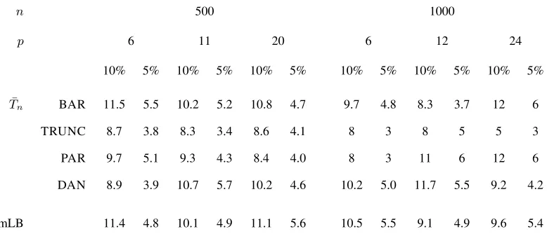
statistic (1). We first investigate the size of the test by considering bivariate standard normal data. Table 1 shows

the achieved levels of all test statistics calculated at5%and10%nominal levels, and indicates that the proposed

test statistics approximate the nominal levels adequately. In order to compare the power of both test statistics, we

Table 1: Empirical type I error (%) of statistics for testing the hypothesis that the data are independent and

identi-cally distributed. The data are generated from the bivariate standard normal distribution. The bandwidthpis[3nλ_],

λ= 0.1,0.2and0.3. Results are based onB= 499bootstrap replications for each of 1000 simulations.

n 500 1000

p 6 11 20 6 12 24

10% 5% 10% 5% 10% 5% 10% 5% 10% 5% 10% 5%

¯

Tn BAR 11.5 5.5 10.2 5.2 10.8 4.7 9.7 4.8 8.3 3.7 12 6

TRUNC 8.7 3.8 8.3 3.4 8.6 4.1 8 3 8 5 5 3

PAR 9.7 5.1 9.3 4.3 8.4 4.0 8 3 11 6 12 6

DAN 8.9 3.9 10.7 5.7 10.2 4.6 10.2 5.0 11.7 5.5 9.2 4.2

mLB 11.4 4.8 10.1 4.9 11.1 5.6 10.5 5.5 9.1 4.9 9.6 5.4

consider a bivariate nonlinear moving average model of order 2,

Xt;i = t;it−1;it−2;i (i= 1,2), (14)

where{t;i, i= 1,2}is an independent and identically distributed sequence of standard normal random variables,

a bivariate generalized autoregressive conditional heteroscedastic model of order(1,1)

Xt;i = h

1/2

t;i t;i (i= 1,2), (15)

where



 

ht;1

ht;2

   =   

0.003

0.005

  +   

0.2 0.1

0.1 0.3

     

Xt2−1;1

X2

t−1;2

  −   

0.4 0.05

0.05 0.5

     

ht−1;1

ht−1;2



 

and{t;i, i= 1,2} is a sample from a bivariate normal with correlationρ= 0.4, and a bivariate autoregressive

model of order 1



 

Xt;1

Xt;2

   =   

0.04 −0.10

0.11 0.50

     

Xt−1;1

Xt−1;2

  +    t;1 t;2  

, (16)

and the error as in the previous model but withρ= 0and0.4. Table 2 shows thatT¯nattains larger power than (1)

when data are generated by the non-linear models (14) and (15). The Ljung–Box test statistic performs better than

¯

Tnwhen data are generated by (16) withρ= 0and for small values ofpand large sample size. Whenpis large,

¯

Tnperforms generally better than (1).

4.4

Application

We analyze monthly unemployment rates of the 50 US states from January 1976 to September 2011, seasonally

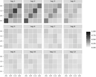
ad-justed and available from Tsay’s (2014) book sitehttp://faculty.chicagobooth.edu/ruey.tsay/ teaching/mtsbk/. We consider first the 416 differenced monthly rates of Alaska, Arkansas, Colorado and Delaware. Figure 1 displays the sample auto-distance correlation matrices at each lag, and reveals the dependence

structure for lags 1 to 12. After the sixth lag, the auto-distance correlation function suggests that there is no

Table 2: Empirical power (%) of all test statistics of size 5%. The bandwidthpis[3nλ],λ= 0.1,0.2and0.3. The results are based onB= 499bootstrap replications for each of1000simulations. The test statisticT¯nis calculated

using the Bartlett kernel.

n 500 800 1000

p 6 11 20 6 12 23 6 12 24

Model (14) ¯

Tn 100 100 100 100 100 100 100 100 100

mLB 40 32.5 26.6 47.1 35.9 28.5 46.6 36.6 26.8 Model (15)

¯

Tn 76.4 79.5 78.3 97.2 98 95.4 99.4 98 99

mLB 56.9 54.6 48.1 65.1 60.4 53.9 64.9 65.2 54.9 Model (16) withρ= 0

¯

Tn 66.6 58.4 44.8 41.3 41.1 69.1 30.4 27 80.4

mLB 48.5 36.1 25.6 75.7 59.4 44.2 86.2 71.8 55.8 Model (16) withρ= 0.4

¯

Tn 71.4 62.5 46.9 92.7 89.7 75.7 96.8 95.6 88

mLB 50.8 37.1 28.3 77.5 58.9 44.6 86.9 72.6 54.1

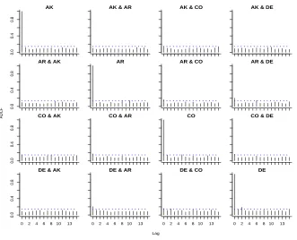
employing the Akaike information criterion, a fifth-order model fits the data well. The auto-distance correlation

plots of the resulting residual series in Figure 2 shows no serial dependence. Tests of independence for the residual

series using the Bartlett kernel for the computation ofT¯nand mLB yieldp-values 0.428, 0.228, 0.158 and 1, 0.999,

lag 9 lag 10 lag 11 lag 12

lag 5 lag 6 lag 7 lag 8

lag 1 lag 2 lag 3 lag 4

AK AR CO DE AK AR CO DE AK AR CO DE AK AR CO DE AK

AR CO DE

AK AR CO DE

AK AR CO DE

0.00 0.25 0.50 0.75 1.00

Figure 1: Visualizing the sample auto-distance correlation matrices of the four-dimensional unemployment series

of Alaska, Arkansas, Colorado and Delaware, starting on top left at lagj = 1. The darker rectangles correspond

AK

0.0

0.4

0.8

AK & AR AK & CO AK & DE

AR & AK

0.0

0.4

0.8

AR AR & CO AR & DE

CO & AK

0.0

0.4

0.8

CO & AR CO CO & DE

DE & AK

0 2 4 6 8 10 13

0.0

0.4

0.8

DE & AR

0 2 4 6 8 10 13

DE & CO

0 2 4 6 8 10 13

DE

0 2 4 6 8 10 13

Lag

ADCF

Figure 2: Auto-distance correlation plot of the residuals vector process after fitting a fifth-order vector

autoregres-sive model to the unemployment data. The dotted horizontal line is drawn following the methodology described in

ACKNOWLEDGMENT

We are grateful to the editor, associate editor and the referees for their insightful comments. We also thank H.

Dehling, G. Székely, M. Rizzo and M. Wendler for useful discussions. Pitsillou’s research was supported by a

University of Cyprus research grant.

A

Appendix

A.1

V

ˆ

rm

(

·

)

as a

V

-statistic

For ease of notation let X ≡ Xt;r andY ≡ Xt+j;m. Suppose thatZi = (Xi, Yi), i = 1, . . . ,6, are

inde-pendent and identically distributed copies of the vectorZ = (X, Y). By Prop. 2.6 of Lyons (2013), define the

function

f(u1, u2, u3, u4) =|u1−u2| − |u1−u3| − |u2−u4|+|u3−u4|,

whereui∈R,i= 1, . . . ,4. Now, set

h(Z1, . . . , Z6) =f(X1, X2, X3, X4)f(Y1, Y2, Y5, Y6). (A.1) Provided thatE(|Xt;r|2)<∞,∀r= 1, . . . , d, we obtain that

Enh(Z1, . . . , Z6)o=E(X1−X2

Y1−Y2 ) +E(

X1−X2 )E(

Y5−Y6 )

−2E(X1−X2

Y1−Y5 )

=V_rm2 (j),

where the last equality follows from Székely et al. (2007, Remark 3). We consider the symmetrized version ofh(·)

given by (A.1), defined as

˜

h(Z1, . . . , Z6) = 1 6!

X

σ∈{1,...,6}

whereσis a permutation of{1, . . . ,6}. Then, we observe that

Enh˜(Z1, . . . , Z6)o= 1 6!

X

σ∈{1,...,6}

Enh(Zσ(1), . . . , Zσ(6))o=V_rm2 (j). Thus, we conclude that the functionV2

rm(j)can be expressed as

V_rm2 (j) =

Z R2 · · · Z R2 ˜

h(z1, . . . , z6)dFrm(z1). . . dFrm(z6).

Because of symmetry and following v. Mises (1947), a biased estimator ofV2

rm(j)is given by

Trm =

1 (n−j)6

n−j X

i1=1

· · · n−j X

i6=1 h

(

(Xi1;r, Xi1+j;m), . . . ,(Xi6;r, Xi6+j;m)

)

= 1

(n−j)6

n−j X

i1=1

· · · n−j X

i6=1

|Xi1;r−Xi2;r| − |Xi1;r−Xi3;r| − |Xi2;r−Xi4;r|+|Xi3;r−Xi4;r|

× |Xi1+j;m−Xi2+j;m| − |Xi1+j;m−Xi3+j;m| − |Xi2+j;m−Xi4+j;m|+|Xi5+j;m−Xi6+j;m|

.

After some calculations, we obtain that

Trm =

1 (n−j)2

n−j X

i1,i2=1

|Xi1;r−Xi2;r| |Xi1+j;m−Xi2+j;m|

+ 1

(n−j)4

n−j X

i1,i2=1

|Xi1;r−Xi2;r|

n−j X

i1,i2=1

|Xi1+j;m−Xi2+j;m|

− 2

(n−j)3

n−j X

i1,i2,i3=1

|Xi1;r−Xi2;r| |Xi1+j;m−Xi3+j;m|

= 1

(n−j)2

n−j X

t,s=1

Ar_tsB_tsm

= Vˆ_rm2 (j),

where the second equality is proved in Székely et al. (2007, Appendix). Because of symmetry we have that

ˆ

V_rm2 (j) =

Z R2 · · · Z R2 ˜

h(z1, . . . , z6)dFˆrm(z1). . . dFˆrm(z6),

whereFˆrm(·)denotes the empirical distribution function defined as

ˆ

Frm(z) =

1 (n−j)

n−j X

t=1

I(Xt;r≤x, Xt+j;m≤y).

Hence, we have shown thatVˆ2

A.2

Derivation of test statistics

Recall that the kernelK(·)satisfies

Assumption A.1K :R→[−1,1]is symmetric and is continuous at 0 and all but a finite number of points, with

K(0) = 1,R_−∞∞ K2_{(z)dz <∞and|K(z)| ≤C|z|}−b

for largezandb >1/2.

Following the notation of the paper, we have that

ˆ

F(ω, u, v) =nfˆ(r,m)(ω, u, v)

od

r,m=1

, Fˆ0(ω, u, v) = 1 2π

n

ˆ

σ(₀r,m)(u, v)

od

r,m=1

,

where

ˆ

f(r,m)(ω, u, v) = 1 2π

(n−1)

X

j=−(n−1)

(1− |j|/n)1/2K(j/p)ˆσ_j(r,m)(u, v)e−ijω (ω∈[−π, π]), (A.3) withK(·)satisfying Assumption A.1 andpis a bandwidth parameter. Consider the squaredL2-distance between

ˆ

F(·,·,·)andFˆ0(·,·,·)

L2₂nFˆ(ω, u, v),Fˆ0(ω, u, v)

o = Z R2 Z π −π

kFˆ(ω, u, v)−Fˆ0(ω, u, v)k2FdωW(du, dv)

= Z R2 Z π −π tr " n ˆ

F(ω, u, v)−Fˆ0(ω, u, v)o

∗

×nFˆ(ω, u, v)−Fˆ0(ω, u, v)o

#

dωW(du, dv).

But,

L22

n

ˆ

F(ω, u, v),Fˆ0(ω, u, v)o = 2

π

X

r,m n−1

X

j=1

(1−j/n)K2(j/p)

Z

R2 σˆ

(r,m)

j (u, v)

2

W(du, dv),

for any suitably weighting functionW(·,·). In particular, employing

W(du, dv) = 1

π|u|2

1

π|v|2dudv, ((u, v)∈R

2_),

yields to

L2₂nFˆ(ω, u, v),Fˆ0(ω, u, v)

o

= 2

π

X

r,m n−1

X

j=1

(1−j/n)K2(j/p) ˆV_rm2 (j)

= 2

π

n−1

X

j=1

In terms of correlation matrices, recall thatD=diag{Vrr(0), r= 1, . . . , d}and define thed×dmatrix

Rj(u, v) =D−1/2Σj(u, v)D−1/2

with elements

ρ(_jr,m)(u, v) = σ (r,m)

j (u, v) {Vrr(0)Vmm(0)}1/2

.

By recalling that

sup_(u,v)∈R2 ∞

X

j=−∞

σ

(r,m)

j (u, v) <∞,

we can define the Fourier transform ofρ(_jr,m)(·,·)by g(r,m)(ω, u, v) = 1

2π ∞

X

j=−∞

ρ(_jr,m)(u, v)e−ijω (ω∈[−π, π]). Define thed×dmatrix

G(ω, u, v) = 1 2π

∞

X

j=−∞

Rj(u, v)e−ijω= n

g(r,m)(ω, u, v)o

d r,m=1.

Under independence,G(·,·,·)reduces to

G0(ω, u, v) = 1 2π

n

ρ(₀r,m)(u, v)o

d r,m=1.

An analogous to (A.3) kernel-density estimator ofg(r,m)_{(·,·)is given by}

ˆ

g(r,m)(ω, u, v) = 1 2π

(n−1)

X

j=−(n−1)

(1− |j|/n)1/2K(j/p) ˆρ_j(r,m)(u, v)e−ijω (ω∈[−π, π]).

We can then define the estimators ofG(·,·,·)andG0(·,·,·)by

ˆ

G(ω, u, v) = nˆg(r,m)(ω, u, v)

od

r,m=1

and

ˆ

G0(ω, u, v) = 1 2π

n

ˆ

ρ(₀r,m)(u, v)o

respectively. Considering now the squaredL2-distance betweenG(·,·,·)andG0(·,·,·)we get

L2₂Gˆ(ω, u, v),Gˆ0(ω, u, v)=

Z

R2 Z π

−π

kGˆ(ω, u, v)−Gˆ0(ω, u, v)k2

FdωW(du, dv)

= Z R2 Z π −π tr " n ˆ

G(ω, u, v)−Gˆ0(ω, u, v)o

∗

×nGˆ(ω, u, v)−Gˆ0(ω, u, v)o

#

dωW(du, dv).

After some calculations and choosing the weighting function defined in (A.4) of the main article, we find that

L2₂Gˆ(ω, u, v),Gˆ0(ω, u, v)

= 2

π

X

r,m n−1

X

j=1

(1−j/n)K2(j/p)

Z

R2 ρˆ

(r,m)

j (u, v)

2

W(du, dv)

= 2

π

X

r,m n−1

X

j=1

(1−j/n)K2(j/p) ˆ

V2

rm(j) {Vˆ2

rr(0) ˆVmm2 (0)}1/2

= 2

π

X

r,m n−1

X

j=1

(1−j/n)K2(j/p) ˆR2_rm(j)

= 2

π

n−1

X

j=1

(1−j/n)K2(j/p)trnRˆ∗(j) ˆR(j)o

= 2

π

n−1

X

j=1

(1−j/n)K2(j/p)trh{Dˆ−1/2Vˆ(j) ˆD−1/2}∗Dˆ−1/2Vˆ(j) ˆD−1/2i

= 2

π

n−1

X

j=1

(1−j/n)K2(j/p)trnVˆ∗(j) ˆD−1Vˆ(j) ˆD−1o.

A.3

Simultaneous critical values

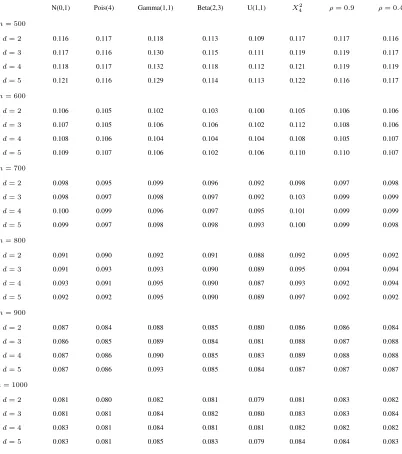
Table 3 illustrates that critical values obtained under independence are not sensitive to the choice of response

dis-tribution or the dimension of a series. They depend on the sample size, as it should be expected. The first six

columns of Table 3 have been obtained by considering univariate independent and identically distributed random

variables. The last two columns correspond to independent samples drawn from ad-dimensional normal

distribu-tion with zero mean and equicorreladistribu-tion matrix with non-diagonal elementsρij=ρ,i6=j. We setρ= 0.9and 0.4

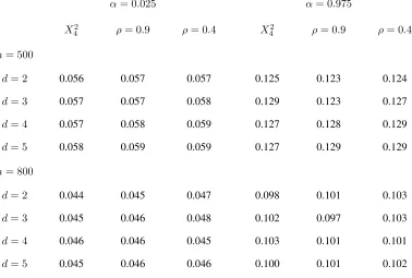
respectively. To further support our argument we include Table 4 which gives critical values for levelsα= 0.025

Table 3: Simultaneous empirical critical values at level α = 0.05, for different sample sizes and dimensions.

Results are based onB = 499bootstrap replications for each of simulations.

N(0,1) Pois(4) Gamma(1,1) Beta(2,3) U(1,1) X2

4 ρ= 0.9 ρ= 0.4

n= 500

d= 2 0.116 0.117 0.118 0.113 0.109 0.117 0.117 0.116

d= 3 0.117 0.116 0.130 0.115 0.111 0.119 0.119 0.117

d= 4 0.118 0.117 0.132 0.118 0.112 0.121 0.119 0.119

d= 5 0.121 0.116 0.129 0.114 0.113 0.122 0.116 0.117

n= 600

d= 2 0.106 0.105 0.102 0.103 0.100 0.105 0.106 0.106

d= 3 0.107 0.105 0.106 0.106 0.102 0.112 0.108 0.106

d= 4 0.108 0.106 0.104 0.104 0.104 0.108 0.105 0.107

d= 5 0.109 0.107 0.106 0.102 0.106 0.110 0.110 0.107

n= 700

d= 2 0.098 0.095 0.099 0.096 0.092 0.098 0.097 0.098

d= 3 0.098 0.097 0.098 0.097 0.092 0.103 0.099 0.099

d= 4 0.100 0.099 0.096 0.097 0.095 0.101 0.099 0.099

d= 5 0.099 0.097 0.098 0.098 0.093 0.100 0.099 0.098

n= 800

d= 2 0.091 0.090 0.092 0.091 0.088 0.092 0.095 0.092

d= 3 0.091 0.093 0.093 0.090 0.089 0.095 0.094 0.094

d= 4 0.093 0.091 0.095 0.090 0.087 0.093 0.092 0.094

d= 5 0.092 0.092 0.095 0.090 0.089 0.097 0.092 0.092

n= 900

d= 2 0.087 0.084 0.088 0.085 0.080 0.086 0.086 0.084

d= 3 0.086 0.085 0.089 0.084 0.081 0.088 0.087 0.088

d= 4 0.087 0.086 0.090 0.085 0.083 0.089 0.088 0.088

d= 5 0.087 0.086 0.093 0.085 0.084 0.087 0.087 0.087

n= 1000

d= 2 0.081 0.080 0.082 0.081 0.079 0.081 0.083 0.082

d= 3 0.081 0.081 0.084 0.082 0.080 0.083 0.083 0.084

d= 4 0.083 0.081 0.084 0.081 0.081 0.082 0.082 0.082

Table 4: Simultaneous empirical critical values at two different s levelsα= 0.025and0.975, for different sample

sizes and dimensions. Results are based onB= 499bootstrap replications for each of 1000 simulations.

α= 0.025 α= 0.975

X42 ρ= 0.9 ρ= 0.4 X42 ρ= 0.9 ρ= 0.4

n= 500

d= 2 0.056 0.057 0.057 0.125 0.123 0.124

d= 3 0.057 0.057 0.058 0.129 0.123 0.127

d= 4 0.057 0.058 0.059 0.127 0.128 0.129

d= 5 0.058 0.059 0.059 0.127 0.129 0.129

n= 800

d= 2 0.044 0.045 0.047 0.098 0.101 0.103

d= 3 0.045 0.046 0.048 0.102 0.097 0.103

d= 4 0.046 0.046 0.045 0.103 0.101 0.101

A.4

Proofs

of Theorem 1 1. Suppose that Vrm2 (j) 6= 0for a fixedj. Recall the notation of Section A.1. The stated

assumptions imply that there exists a positive numberδsuch that forν= 2 +δthe following statements are

true:

i. En

˜

h(Z1, . . . , Z6)

νo

<∞,

ii. sup_i1<···<i6En

˜

h(Zi1_{, . . . , Z}i6₎

νo

<∞.

Their verification is based on the proof of (Lyons, 2013, Prop. 2.6) and the form of the kernel given by (A.2).

Hence, we conclude that

n1/2

ˆ

V_rm2 (j)−V_rm2 (j)

→ N(0,36σ2), with

σ2=E{˜h2₁(Z1)} −V_rm4 (j)+ 2

"_∞ X

k=1

E{˜h2₁(Z1)˜h₁2(Zk+1)} −V_rm4 (j)

#

, (A.4)

where˜hc(z1, . . . , zc)denotes the conditional expectation of˜h(·)defined as:

˜

hc(z1, . . . , zc) =E n

˜

h(z1, . . . , zc, Zc+1, . . . , Z6)o (c= 1, . . . ,5). The above result follows directly from Yoshihara (1976, Thm. 1).

2. Considering now the case where the data are pairwise independent, we observe that

h1(z1) =Enh(z1, Z2, . . . , Z6)o= 0,

which implies that˜h1(z1) = 0, almost sure. The latter shows that theV–statisticVˆrm2 (j)has a degeneracy

of order 1. The statisticVˆrm2 (·)can be decomposed as (Hoeffding, 1948; Sen, 1972; Yoshihara, 1976)

ˆ

V_rm2 (j) =

₆

2

V_n(2)+Rn, (A.5)

whereRn =OP(n1+γ),γ >2.V

(2)

the ’centered’ version of˜h2(z1_{, z}2_{)given by (Serfling, 1980, p. 222)} ˜

h(2)(z1, z2) = ˜h2(z1, z2)− Z

R2

˜

h2(z1, z2)dFrm(z1)− Z

R2

˜

h2(z1, z2)dFrm(z2)

+

Z

R2 Z

R2

˜

h2(z1, z2)dFrm(z1)dFrm(z2),

such that

V_n(2)=

Z

R2 Z

R2

˜

h(2)(z1, z2)dFˆrm(z1)dFˆrm(z2). (A.6)

Under pairwise independence,˜h(2)(z1, z2) = ˜h2(z1, z2)almost surely. We further observe thath2(z1_{, z}2_{) =E}n_h(z1_{, z}2_{, Z}3_{, . . . , Z}6₎o_=d

X(x1, x2)dY(y1, y2)by recalling that

foru, u0∈RandXa real valued random variable

mX(u) =E(|X−u|), m¯X =E{mX(X)}, dX(u, u0) =|u−u0| −mX(u)−mX(u0) + ¯mX.

In addition,

˜

h2(z1, z2) =En˜h(z1, z2, Z3, . . . , Z6)o=

₆

2

−1

h2(z1, z2). Thus, (A.5) and (A.6) show that

ˆ

Vrm2 (j) = ₆

2

₆

2

−1 ₁

(n−j)2

n−j X

t,s=1

h2(zt, zs) +Rn

= 1

(n−j)2

n−j X

t,s=1

dX(Xt;r, Xs;r)dY(Yt;m, Ys;m) +Rn.

ButnRn →0, in probability, asn→ ∞. Therefore,

nVˆ_rm2 (j)−1

n

n−j X

t,s=1

dX(Xt;r, Xs;r)dY(Yt;m, Ys;m)→0,

in probability, as n → ∞. In addition, under pairwise independence, we have that Enh2(z, Zs) |

Z1_{, . . . Z}s−1o_{= 0almost surely. Therefore applying Theorem 1 of Leucht and Neumann (2013a) shows}

that

1

n

n−j X

t,s=1

dX(Xt;r, Xs;r)dY(Yt;m, Ys;m)→Z = X

l

λlZl2,

Define

¯

f(r,m)(ω, u, v) = 1 2π

(n−1)

X

j=−(n−1)

K(j/p)(1− |j|/n)1/2σ˜(_jr,m)(u, v)e−ijω,

where

˜

σ(_jr,m)(u, v) = 1

n− |j| n X

t=|j|+1

ψt;r(u)ψt−|j|;m(v) (A.7)

and

ψt;r(u) ≡ eiuXt;r−φ(r)(u). (A.8)

The corresponding pseudoestimator of the generalized spectral density matrix is defined as

¯

F(ω, u, v) = 1 2π

(n−1)

X

j=−(n−1)

K(j/p)(1− |j|/n)1/2Σ˜_|j|(u, v)e−ijω,

whereΣ˜|j|(·,·) is the covariance matrix ofeiuXt with elements given by (A.7). For the proof of Theorem 2, we will need the following two lemmas whose proof is omitted as it follows closely the arguments given in the

supplementary material of Fokianos and Pitsillou (2017) and the fact thatβ-mixing impliesα-mixing.

Lemma A.4.1Let {Xt} be a β-mixing strictly stationary process with mixing coefficients satisfying β(k) =

O(k−2_{). Suppose thatE|Xt,r|}2

<∞,r= 1, . . . , d. Then we have that

(n−j)2E

σˆ

(r,m)

j (u, v)−σ˜

(r,m)

j (u, v)

2

≤ Cand(n−j)E

σ˜

(r,m)

j (u, v)

2

≤Cuniformly in(u, v)∈ R2for r, m= 1, . . . , p.

Lemma A.4.2Let {Xt} be a β-mixing strictly stationary process with mixing coefficients satisfying β(k) =

O(k−2_{). Suppose that E|Xt,r|}2

< ∞, r = 1, . . . , d. For each γ > 0, letD(γ) = {(u, v) : γ ≤ |u| ≤

1/γ, γ≤ |v| ≤1/γ}. Then

Z

D(γ)

n−1

X

j=1

K2(j/p)(n−j) σˆ

(r,m)

j (u, v) 2 − ˜σ

(r,m)

j (u, v)

2

W(du, dv) = OP(p/ √

n)

= oP( √

p)

of Theorem 2 It can be shown that (Hong (1999))

n−1

X

j=1

K2(j/p)(n−j) ˜σ

(r,m)

j (u, v)

2

= Cˆrm(u, v) + ˆVrm(u, v) (A.9)

where

ˆ

Crm(u, v) =

n−1

X

j=1

K2_(j/p)

n−j

 

 n X

t=j+1

C_ttjrm(u, v)

 



,

ˆ

Vrm(u, v) =

n−1

X

j=1

K2_(j/p)

n−j

 

 n X

t=j+2

t−1

X

s=j+1

V_tsjrm(u, v)

 



,

with

V_tsjrm(u, v) = C_tsjrm(u, v) +C_stjrm(u, v)∗

and

C_tsjrm(u, v) = ψt;r(u)ψs;r(u)∗ψt−j;m(v)ψs−j;m(v)∗,

where∗denotes complex conjugate.

For the first summand of (A.9), it holds thatR_D(γ)C_ttjrm(u, v)W(du, dv)andR_D(γ)C_ssjrm(u, v)W(du, dv)are inde-pendent integrals unlesst=sors±j. In addition,

E

Z

D(γ)

C_ttjrm(u, v)W(du, dv) = C₀rmγ ≡ Z

D(γ)

σ₀(r,r)(u,−u)σ₀(m,m)(v,−v)W(du, dv)<∞,

shows thatEhPn_t=j+1nR D(γ)C

rm

ttj(u, v)dW −C rmγ

0

oi2

≤C(n−j).Hence, by Markov’s inequality,

Cauchy-Schwarz inequality and the properties of the kernel function, we obtain that

Z

D(γ) ˆ

Crm(u, v)dW = OP(p/ √

n) +C₀rmγ

n−1

X

j=1

So, using Lemma A.4.2, equations (A.9) and (A.10) we have the following:

Z

D(γ)

nn_X−1 j=1

K2(j/p)(n−j) σˆ

(r,m)

j (u, v)

2o

W(du, dv)

=

Z

D(γ)

nn_X−1 j=1

K2(j/p)(n−j) σ˜

(r,m)

j (u, v)

2o

W(du, dv) +OP(p/ √

n)

=

Z

D(γ) ˆ

Crm(u, v)W(du, dv) +

Z

D(γ) ˆ

Vrm(u, v)W(du, dv) +OP(p/ √

n)

=C₀rmγ

n−1

X

j=1

K2(j/p) + ˆV_nrmγ+OP(p/ √

n),

whereVˆrmγ n ≡

R D(γ)Vˆ

rm_{(u, v)W(du, dv). Therefore}

T_n(r,m_;γ ) ≡ Z

D(γ)

nn_X−1 j=1

K2(j/p)(n−j) σˆ

(r,m)

j (u, v)

2o

W(du, dv)

= C₀rmγ

n−1

X

j=1

K2(j/p) + ˆV_nrmγ+OP(p/ √

n). (A.11)

Given Assumption A.1 and by applying Hong (1999, Thm. A.3) onD(γ), we obtain

ˆ

V_nrmγ = Vˆ_ngrmγ+oP( √

p) (A.12)

where

ˆ

V_ngrmγ =

n X

t=g+2

t−g−1

X

s=1

g X

j=1

K2_(j/p)

n−j

Z

D(γ)

V_tsjrm(u, v)W(du, dv)

andg ≡ g(n)such thatg/p → 0, g/n → 0. Now, by applying Hong (1999, Thm. A.4) onD(γ)we get the

following:

n

pD₀rmγ

Z ∞

0

K4(z)dzo −1/2

ˆ

Vngrmγ → N(0,1) (A.13)

asn→ ∞in distribution, where

Drmγ₀ = 2

Z

D(γ)

σ

(r,r) 0 (u, u0)σ

(m,m) 0 (v, v0)

2

Equations (A.11), (A.12) and (A.13) yield to

R

D(γ)

n

j=1 K

2_(j/p)(n−j) σˆ

(r,m)

j (u,v)

2

o

W(du,dv)−C₀rmγPn−1

j=1 K 2_(j/p)

n

pD₀rmγR∞ 0 K

4_(z)dz

o

→

N

(0

,

1)

,

asn→ ∞, in distribution.

Observe thatCˆ₀rmγ −C₀rmγ = OP(1/ √

n)and thatDˆ₀rmγ → Drmγ₀ in probability. Moreover, under Assump-tion A.1, p → ∞andp/n → 0, p−1Pn_j=1−1K2(j/p) = R₀∞K2(z)dz+O(p−1/2). Thus, one can replace C₀rmγPn_j=1−1K2_(j/p)byCˆrmγ

0 p

R

K2_{(z)dz. Summarizing, (A.14) becomes}

Tn(r,m;γ )−Cˆ₀rmγpR₀∞K2(z)dz n

pDˆ₀rmγR∞

0 K

4_(z)dzo1/2

→ N(0,1).

The rest of the proof follows by similar arguments given in Fokianos and Pitsillou (2017), by showing that

lim sup

γ→0

lim sup

n→∞

T

(r,m)

n −T

(r,m)

n;γ

= 0. (A.15)

of Corollary 1 We only show the proof of the first result. From Theorem 2 and under the null hypothesis of

independence, the random variablesTn(r,m)satisfy

Tn(r,m)−Cˆ₀rmγpR₀∞K2(z)dz (

pDˆrmγ₀ R∞

0 K 4_(z)dz

)1/2 → N(0,1) (A.16)

in distribution, asn→ ∞, forr, m= 1, . . . , d. Following similar arguments analogous to the proof of Theorem

2, it can be shown that

X

r,m Z

D(γ)

nn_X−1 j=1

K2(j/p)(n−j) σˆ

(r,m)

j (u, v)

2o

W(du, dv) = X

r,m

C₀rmγ

n−1

X

j=1

K2(j/p)

+ X

r,m

ˆ

V_nrmγ+OP(p/ √

n).

Given Assumption A.1 and employing similar arguments to those of Hong (1999, Proof of Thm. A3), we obtain

that

X

r,m

ˆ

V_nrmγ = X

r,m

ˆ

V_ngrmγ+oP( √

where

ˆ

V_ngrmγ =

n X

t=g+2

t−g−1

X

s=1

g X

j=1

K2_(j/p)

n−j

Z

D(γ)

V_tsjrm(u, v)W(du, dv)

andg≡g(n)such thatg/p→0, g/n→0. Considering the definition ofV_tsjrm(u, v)we obtain that

ˆ

V_ngγ =

n X

t=g+2

" g X

j=1

t−g X

s=1

K2_(j/p) (n−j)

Z

D(γ)

X

r,m n

ψt;r(u)ψt+j;m(v)ψs;r(−u)ψs+j;r(−v) o

W(du, dv)

+

g X

j=1

t−g X

s=1

K2_(j/p) (n−j)

Z

D(γ)

X

r,m n

ψt;r(−u)ψt+j;m(−v)ψs;r(u)ψs+j;r(v) o

W(du, dv)

#

From (A.8), we observe thatnP

r,mψt;r(u)ψt+j;m(v) o

andnP

r,mψs;r(u)ψs+j;m(v) o

are independent fort−

s > gand1≤j≤g. Thus, by applying Hong (1999, Thm. A4) we obtain that

nX

r,m

pDrmγ₀

Z ∞

0

K4(z)dzo

−1/2_X

r,m

ˆ

V_ngrmγ → N(0,1)

asn→ ∞in distribution. Thus, we get the required result onD(γ). Then, following the same arguments as in the

proof of Theorem 2, we finally get the following result

˜

Mn =

P r,mT

(r,m)

n −

P r,mCˆ

rmγ

0

pR₀∞K2(z)dz

(

P r,mDˆ

rmγ

0

pR₀∞K4_(z)dz

)1/2 → N(0,1),

in distribution, asn→ ∞.

For the second result, recall thatT¯n(r,m)may be written as

¯

T_n(r,m) = 1

ˆ

Vrr(0) ˆVmm(0)

T_n(r,m).

By recalling result (A.16), we get

¯

Tn(r,m)−cˆ(0r,m)p

R∞

0 K 2_(z)dz

(

ˆ

d(₀r,m)pR∞

0 K4(z)dz

)1/2 →N(0,1),

in distribution, asn→ ∞, forr, m= 1,2, . . . , d, where

ˆ

c(₀r,m)= ˆ

C₀(r,m)

ˆ

Vrr(0) ˆVmm(0)

, dˆ(₀r,m)= ˆ

D(₀r,m)

ˆ

V2

rr(0) ˆVmm2 (0)

Butdˆ(₀r,m)→2almost surely. Following the same methodology as before, we get that

¯

Mn=

¯

Tn−

P r,mcˆ

(r,m) 0

pR∞

0 K 2_(z)dz

d

(

2pR∞

0 K 4_(z)dz

)1/2 → N(0,1),

in distribution, asn→ ∞and the proof is now completed.

of Theorem 3 We prove the first result of the theorem. RecallD(γ)defined in Lemma 2. For the proof we show

the following: (i)ER_D(γ)R₋π_π

ˆ

f(r,m)(ω, u, v)−f(r,m)(ω, u, v)

2

dωW(du, dv) →0which is proved similarly

to the proof of Hong (1999, Proof of Thm. 2, p. 1213) on D(γ) for allr, m = 1, . . . , dgiven that {Xt} is aβ-mixing strictly stationary, but not independent and identically distributed process, with mixing coefficients

satisfyingP

kβ(k) <∞and the kernel function satisfies assumption A.1. Additionally, by applying Markov’s

inequality we get (ii)Cˆ₀rmγ=OP(1)and (iii)Dˆ rmγ

0 →D

rmγ

0 in probability.

The last remark together with assumption A.1 shows that

1

p1/2

nX

r,m

ˆ

D₀rmγp

Z ∞

0

K4(z)dzo

1/2

→ nX

r,m

Drmγ₀

Z ∞

0

K4(z)dzo

1/2

,

in probability. Using remarks (i) and (ii) and after some calculations we get that

1

n

n

Tn;γ− X

r,m

ˆ

C₀rmγ

Z ∞

0

K2(z)dzo → π

2L 2 2;γ

n

F(ω, u, v), F0(ω, u, v)o, in probability, where

Tn;γ = X

r,m

T_n(r,m_;γ ), and

L22;γ n

F(ω, u, v), F0(ω, u, v)o =

Z

D(γ)

Z π

−π

tr

" n

F(ω, u, v)−F0(ω, u, v)o

∗

×nF(ω, u, v)−F0(ω, u, v)o

#

dωW(du, dv).

References

Aaronson, J., R. Burton, H. Dehling, D. Gilat, T. Hill, and B. Weiss (1996). Strong laws for L- and U-statistics.

Trans. Am. Math. Soc.348, 2845–2866.

Benjamini, Y. and Y. Hochberg (1995). Controlling the false discovery rate: A practical and powerful approach. J.

R. Stat. Soc. Series B57, 289–300.

Borovcova, S., R. Burton, and H. Dehling (1999). Consistency of the Takens estimator for the correlation

dimen-sion.Ann. Appl. Probab.9, 376–390.

Brockwell, P. J. and R. A. Davis (1991). Time Series : Theory and Methods. New York: Springer-Verlag. Second

Edition.

Chen, B. and Y. Hong (2012). Testing for the Markov property in time series. Econ. Theory28, 130–178.

Chen, X. (2016). Gaussian approximation for the sup-norm of high-dimensional matrix-variate U-statistics and its

applications. availabe at http://arxiv.org/abs/1602.00199.

Chwialkowski, K. P., D. Sejdinovic, and A. Gretton (2014). A wild bootstrap for degenerate kernel tests. In

Z. Ghahramani, M. Welling, C. Cortes, N. Lawrence, and K. Weinberger (Eds.),Advances in Neural Information

Processing Systems 27, pp. 3608–3616.

Davis, R. A., M. Matsui, T. Mikosch, and P. Wan (2016). Applications of distance correlation to time series.

Bernoulli. to appear.

Dehling, H. and T. Mikosch (1994). Random quadratic forms and the boostrap for U-statistics. J. Multivar.

Anal.51, 392–413.

Dueck, J., D. Edelmann, T. Gneiting, and D. Richards (2014). The affinely invariant distance correlation.

Bernoulli20, 2305–2330.

Fokianos, K. and M. Pitsillou (2017). Consistent testing for pairwise dependence in time series.Technometrics59,

262–270.

Gretton, A., K. Fukumizu, C. H. Teo, L. Song, B. Schölkopf, and A. Smola (2008). A kernel statistical test of

independence.Adv. Neural. Inf. Process. Syst.20, 585–592.

Hipel, K. W. and A. I. McLeod (1994). Time Series Modelling of Water Resources and Environmental Systems.

Amsterdam: Elsevier Science Pub Co.

Hlávka, Z., M. Hu˘sková, and S. G. Meintanis (2011). Tests for independence in non-parametric heteroscedastic

regression models.J. Multivar. Anal.102, 816–827.

Hoeffding, W. (1948). A class of statistics with asymptotically normal distribution.Ann. Math. Stat.19, 293–325.

Hong, Y. (1998). Testing for pairwise serial independence via the empirical distribution function. J. R. Stat. Soc.

Series B60, 429–453.

Hong, Y. (1999). Hypothesis testing in time series via the emprical characteristic function: A generalized spectral

density approach. J. Am. Stat. Assoc.94, 1201–1220.

Hong, Y. (2000). Generalized spectral tests for serial dependence. J. R. Stat. Soc. Series B62, 557–574.

Hosking, J. R. M. (1980). Multivariate Portmanteau statistic. J. Am. Stat. Assoc.75, 349–386.

Lacal, V. and D. Tjøstheim (2017). Local Gaussian autocorrelation and tests of serial independence. J. Time. Ser.

Anal.38, 51–71.

Lacal, V. and D. Tjøstheim (2018). Estimating and testing nonlinear local dependence between two time series. J.

Bus. Econ. Stat.. to appear.

Leucht, A. and M. H. Neumann (2013a). Degenerate U- and V-statistics under ergodicity: asymptotics, bootstrap