Real Time Scalable Visual Tracking via Quadrangle Kernelized Correlation Filters

Real-Time Scalable Visual Tracking via Quadrangle

Kernelized Correlation Filters

Guiguang Ding, Wenshuo Chen, Sicheng Zhao, Jungong Han, Qiaoyan Liu

Abstract—Correlation filter (CF) has been widely used in tracking tasks due to its simplicity and high efficiency. How-ever, conventional CF based trackers fail to handle the scale variation occurs when the targeted object is moving, which is one of the most notable unsolved problems of visual object tracking. In this paper, we propose a scalable visual tracking algorithm based on kernelized correlation filters, referred to as Quadrangle Kernelized Correlation Filters (QKCF). Unlike existing complicated scalable trackers that either perform the correlation filtering operation multiple times or extract many candidate windows at various scales, our tracker intends to estimate the scale of the object based on the positions of its four corners, which can be detected using a new Gaussian training output matrix within one filtering process. After obtaining four peak values corresponding to the four corners, we measure the detection confidence of each part response by evaluating its spatial and temporal smoothness. On top of it, a weighted Bayesian inference framework is employed to estimate the final location and size of the bounding box from the response matrix, where the weights are synchronized with the calculated detection likelihoods. Experiments are performed on the OTB-100 dataset and 16 benchmark sequences with significant scale variations. The results demonstrate the superiority of the proposed method in terms of both effectiveness and robustness, compared to the state-of-the-arts.

Index Terms—Image emotion, probability distribution, valence-arousal, Gaussian mixture model, shared sparse regression, multi-task learning

I. INTRODUCTION

With the rapid development of digital multimedia technol-ogy, the total amount of video data, such as user-generated videos and surveillance videos, has been explosively increas-ing, which poses a great challenge to Internet inspection and security monitoring. As an important technique in computer vision, visual object tracking [1], [2] aims to estimate the location of a visual target at each frame of an image sequence and plays an important role in intelligent transportation sys-tems [3], [4]. Due to the complexity of real-world scenes, such as illumination variation, partial occlusion, background

Copyright (c) 2013 IEEE. Personal use of this material is permitted. However, permission to use this material for any other purposes must be obtained from the IEEE by sending a request to [email protected]. Manuscript received March 30, 2017. This work was supported by the National Natural Science Foundation of China (No. 61571269, 61671267, 61701273), China Postdoctoral Science Foundation (No. 2017M610897), and the Royal Society Newton Mobility Grant (IE150997). Corresponding authors: Jungong Han; Sicheng Zhao

G. Ding, W. Chen, S. Zhao and Q. Liu are with the School of Software, Tsinghua University, Beijing 100084, China (e-mail: [email protected]; [email protected]; [email protected]; [email protected]).

J. Han is with School of Computing and Communications, Lancaster University, Lancaster, LA1 4YW, UK (e-mail: [email protected]).

——Ours ——KCF

Fig. 1. Comparisons of the proposed QKCF with KCF tracker [5] in the challenging situation of scale variation on theCarScalesequence [6]. While preserving the high tracking speed of KCF, our tracker can well handle the scale variation problem by a Gaussian training output matrix with four peak values in one filter.

clutter, motion blur and scale variation, visual tracking remains a challenging task.

the object-scale variation for most practical situations, the computational efficiency is dramatically degraded due to the multiple filtering operations carried out in one single frame.

In this paper, we aim to solve the scale variation problem in a single-frame-single-filter framework. Based on the intrinsic boundary extension property of CF trackers, we introduce a quadrangle Gaussian training label matrix to fully explore the boundary information of the target object. By improving the training and tracking algorithms of KCF [5], we propose Quadrangle Kernelized Correlation Filters (QKCF), which can simultaneously obtain the location and scale of the target object in only one filter.

The CF trackers usually train a model based on the labeled bounding box of the target object in the first frame and then determine the offset location of the target object in subsequentl frames by CF operations, which is called target translation detection. Without taking the scale variation into consideration, the traditional KCF tracker [5] only requires obtaining the centre point of the target object, which can be easily accomplished by selecting the offset with the maximum response. However, the proposed quadrangle Gaussian training label matrix relies on the boundary information instead of the centre point. Therefore, a straightforward duplication of maximum response will no longer work in this context.

To tackle this problem, a weighted Bayesian inference framework is proposed to estimate the location and size of the bounding box from the four-peak-value response matrix. More specifically, it adaptively measures each part response both spatially and temporally, and then makes a biased combination of all confidence maps based on the response weights. In practice, some parts of the object may be occluded or undergo illumination changes, thereby producing unreliable informa-tion. In our formulation, we adaptively adjust the weights such that the information from unreliable parts contributes less during the combination. We conduct extensive experiments on the OTB-100 dataset and 16 benchmark sequences with sig-nificant scale variations. The experimental results demonstrate the superiority of the proposed method in terms of tracking accuracy, efficiency and robustness, compared to the state-of-the-art tracking methods.

The rest of this paper is organized as follows. Section II reviews related work on visual tracking. The detailed algo-rithms, i.e., the quadrangle kernelized correlation filter and weighted Bayesian inference are described in Section III and Section IV, respectively. Experimental evaluation and analysis are presented in Section VI, followed by conclusion and future work in Section VII.

II. RELATEDWORKS

Visual tracking has been extensively studied and numerous trackers [1], [2], [6], [19] have been proposed in the past decade. In this section, we briefly discuss the methods closely related to our work, which are (i) CF based trackers and (ii) scalable visual trackers.

Correlation filter based trackers:As a popular measurement of the correlation or similarity between two signals, correlation filter (CF) has been widely used in various applications, such

as eye localization and object detection [20]. Since the CF operator can be easily transferred into the Fourier domain, on which the correlation can be efficiently computed via FFT, CF-based trackers have been widely used in real-time applications [5], [7]–[10]. Having initialized a small window centered on the object in the first frame, the target is tracked by correlating the filter over a larger searching window in next frame and the new location of the target is specified by looking at the maximum correlation response. This new location is in turn used to updated the filter.

MOSSE [7] is the first CF based tracker, which directly takes the gray values as visual features and detects the target object via a linear CF classifier. The tracking speed of MOSSE can reach several hundreds frames per second with the aid of CF. Heriques et al. proposed extending CF to a kernel space by the CSK method [8], which is built upon the illumination intensity features. Both KCF tracker [5] and CAT tracker [9] are the extended multi-channel versions of CSK, where the former one adopted the geometry and illumination invariant HOG features while the latter replaced the original gray scale representation with the color attributes. Zhang et al. [10] changed the Gaussian function in MOSSE to a Bayesian framework such that the contextual information can be incorporated into the filter learning. This STC track can model the scale change to limited extent based on consecutive correlation responses. To sum up, all the above methods are restricted to only estimating the target translation so that they generally yield a poor performance in complex scenarios where significant scale changes occur.

Deep trackers: Very recently, owing to the powerful fea-ture learning capability of CNN, deep networks have been introduced into visual tracking. Due to lacks of training data, CNNs are usually pretrained on a large-scale dataset for image classification [23] [24] [25] [26] to learn a generic relationship between object motion and appearance in either an on-line or off-line manner. Late on, [27] [28] [29] propose to train the CNNs on a set of annotated video sequences instead of still images, and the obtained results showed that the CNNs trained on video sequences are more robust to the environmental variations. In contrast to these deep trackers that reply on a large training set, our algorithm aims to tracking scaling objects based on fast CF technique with no need for an intensive training procedure.

It is noted that there are some other tracking methodologies related to our research, including tracking-by-detection [12], [22], ensemble tracking [30]–[33], contour tracking [34], [35], hash tracking [36], multi-cue tracking [37] and multi-object tracking [38]–[42]. Tracking-by-detection algorithms [12], [22] base their trackers on the object detection results. Dif-ferently, ensemble tracking [30]–[33] combines a set of weak classifiers, which are trained online to distinguish the object from background, into a strong classifier to label pixels in the next frame. Contour tracking [34], [35] aims to track the fine-grained contours instead of simple rectangles, which is often used for non-rigid objects. Hash tracking maps the high-dimensional data to a compact binary code, solving the scale and dimension increasing problem with a constant time. Multi-cue tracking [37] jointly employs different cues about the object for the accurate localization of target object in extreme conditions, while multi-object tracking [38]–[42] tracks multiple objects simultaneously. The proposed QKCF can be deemed as one kind of tracking-by-detection trackers but with high accuracy and fast speed. Distinct from ensemble tracking, contour tracking, hash tracking, multi-cue tracking and multi-object tracking, the proposed method is a non-ensemble, non-contour, single-cue and single-object tracker.

III. QUADRANGLEKERNELIZEDCORRELATIONFILTER

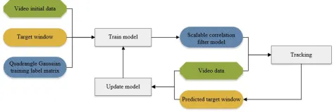
Basically, we aim to build a real-time tracking system that is robust to scale variations, and meanwhile, avoid using time-consuming multi-sampling strategy or multi-scale space pyra-mid. Due to the high efficiency and competitive performance of KCF [5], we base our method on the KCF tracker. The key idea is to employ a Gaussian training output matrix with four peak values to implement multiple edges tracking in one filter operation. Furthermore, a weighted Bayesian inference framework is proposed to deduce the location and size of the bounding box simultaneously. The flowchart despicting the whole process is shown in Figure 2

A. The KCF Tracker

In this section, we briefly introduce the KCF tracker. More details can be referred to [5]. Using the ridge regression as a filtering model, KCF aims to find a function f(z) = wTz that minimizes the squared error over samples xi and their

Fig. 2. Flowchart of QKCF process. At the first frame, initial frame data and the groundtruth are used to train the first correlation filter model. After predicting the target window of the next frame by the model, we use the frame data and the target window to update the model, and then predict the next frame again.

regression targetsyi,

min

w

X

i

(f(xi)−yi)2+λkwk2, (1)

where w is kernelized filtering template and λ is a regular-ization parameter that controls overfitting. Suppose the kernel function isκ(x,x0) =hϕ(x), ϕ(x0)i. After mapping the inputs of a linear problem to a nonlinear feature-space ϕ(x), the closed form solution of ridge regression is

w=X

i

αiϕ(xi). (2)

Based on the circulant matrix structure and Convolution The-orem, vectorα can be obtained by

α=F−1

_F(y)

F(k) +λ

, (3)

whereFandF−1_{denote the Fourier transform and its inverse,}

respectively; k is a row vector of the n×n kernel matrix K. Following the settings in KCF [5], the Gaussian kernel is adopted κ(x,x0) = exp(−kx−x0k2_/σ2_{). Andk is computed}

by

k= exp

− 1 σ2 kxk

2_+kx0_k2_−2F−1_(F∗_(x)·F(x0₎₎

, (4)

where F∗_{(x) is the conjugate of the Fourier transform. The}

complexity of computing a full kernel correlation isO(nlogn)

[5].

When tracking the object in subsequent frames, suppose the HOG feature of the candidate window isz, the confidence score is calculated as

yz=

X

i

αiκ(z,xi), (5)

whereκ(z,xi)is the kernel distance between regression sam-plezand training samplexi. SupposeKz is the kernel matrix composed of the kernel distance between all training samples and all candidate windows, it has been proved that Kz is a circulant matrix and the circulant basis iskxz.

Similar to training, for the densely sampled candidate windows based on z, we can obtain the following efficient computation based on convolution theorem

11 12 13 ⋯ 1 1 1

21 22 23 ⋯ 2 1 2

31 32 33 ⋯ 3 1 3

⋮ ⋮ ⋮ ⋮ ⋮ ⋮

1 1 1 2 1 3 ⋯ 1 1 1

1 2 3 ⋯ 1

Fig. 3. The Gaussian training label matrix used in QKCF.

where f(z) contains the detection results of all the offset transform to candidate window (z). The responses of all candidate offsets can be obtained by only one computation.

B. Quadrangle Gaussian training label matrix

In a traditional KCF, the Gaussian training label matrix y used to train the filtering template is composed of the training labels with different offsets of the training samples. The(i, j)

element yij is the label score of the offset window withi−1 steps (pixels if grey scale feature is used and cells if HOG is used) downwards and j−1 steps rightwards offset, while y11 corresponds to the original location of the target without

offset. Gaussian function is adopted to representyin KCF [5]. When training the tracking model in the first frame, only the zero-offset window is used as a positive sample.

However, since KCF tracker uses a target-centered window as the training sample, it can only detect the offset of the target between the current frame and previous one. It is unable to detect the scale variation when target expands or shrinks visually because its tracking model is not trained that way. To keep it simple, KCF [5] does not determine the scale variation besides the location. PBT tracker [16], LCT tracker [17] and DSST tracker [18] are CF-based trackers to solve the scale variation problem, but all of them choose to sacrifice speed advantage by sampling, training and filtering the candidate windows multiple times.

To solve the scale variation problem under KCF tracker’s one-sampe-one-filter framework, we redefine the Gaussian training label matrix yby incorporating the edge information of the target into the tracking model. Instead of only using the zero-offset (target-in-center) window as the positive sample, the offset images in the four window corners of the target are also considered as positive samples to determine the target edges. As shown in Figure 3, the four elementsy22,y2(n−1),

y(m−1)2 and y(m−1)(n−1) indicate the training response of

the target-at-right-down-corner (right-down for short) window, left-down window, right-up window and the left-up window, respectively. By redefining the training matrix y, we do not need to extract the four windows, because their corresponding elements in ywill help do the work when filtering.

Formally, suppose the circulant offset between the four cornered training samples and the original sample are ∆1 = (i1, j1), ∆2= (i2, j2),∆3= (i3, j3),∆4 = (i4, j4), then the

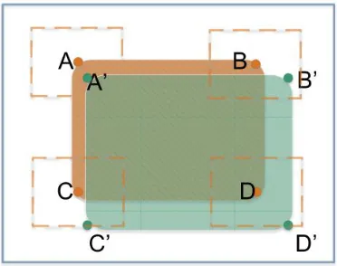
Fig. 4. Examples of quadrangle edge tracking.Rectangle ABCD is location of the current target, while A’B’C’D’ refers to target window of the next frame. The hollow blue rectangle represents the actual extended filter template. Nonzero areas of label matrix are shown as four dashed boxes.

matrixy can be calculated by

y= 4 X

i=1

GL(_by)⊕∆i, (7)

where GL(_by) transforms the zero matrix_by to a single peak Gaussian matrix where the single peak appears on the upper left_by11,⊕represents the circulant offset operation to a matrix.

Inputting the redefined Gaussian training label matrix y into the tracking model allows us to train the KCF with the aim to obtain the four edged offset images. The size and location of the target can thereby be determined by utilizing the relative offset of the adjacent edged images.

As shown in Figure 4, rectangle ABCD represents the location of target in the current frame, while A’B’C’D’ refers to the its location in the next frame. It can be seen from the picture that the target moves towards right bottom direction and becomes a little larger.

The hollow blue rectangle represents the actual extended filter template. In the training stage, we use the patch cropped by blue rectangle to train the filter. The positive samples whose value are 1 locate at the very center of four corners of ABCD. To be more specifically, the whole label matrix y is defined by four accumulative Gaussian matrices. Here, nonzero areas are shown as four dashed boxes.

In detection, the detecting window is still the blue rectangle. We first get all the candidate windows by circulant dense matrices, which will be scanned via the filter we obtained in the training procedure. The one with the highest score is chosen as the final target of the current frame. According to the responsive matrix, we can now calculate the exact coordinates of the four border lines of the target rectangle. The detailed inference is provided in the next section.

IV. WEIGHTEDBAYESIANINFERENCE

A scheme is needed to measure the confidence score of each partial tracking result based on both temporal and spatial information, and on top of it, a combining mechanism that determines the optimal target window by analysing multiple peak filtering results, each being elaborated below.

A. Spatio-Temporal Confidence Score of Partial Filter Re-sponse

Using the quadrangle Gaussian training label matrix yand the trained filter templateF(α), we can obtain the quadrangle filter response matrix f(z). In order to evaluate the filter response of each part, based on the circulant offset of f(z)

with distance ∆i = (ii, ji), we capture local response matrix ri with width and height sfrom the migrated matrix by

ri= (f(z)⊕∆i)

−s

2 :

s

2

. (8)

Temporally, the movement of the target between two adja-cent frames should not be large. As a result, we simply exploit filter response displacement to measure the smoothness of the tracking results between two frames for each part

SCi =krti−r t−1

i k, (9)

whererti andr t−1

i are the filter response matrix of theith part in the tth and t−1th frame.

Spatially, we use peak-to-sidelobe ratio (PSR) to measure the confidence score of the filter response peak to other candidate windows in the current frame, which is defined as

P SRi=

max(ri)−µi σi

, (10)

where µi and σi are the average and standard deviation of ri, respectively. By jointly combining SCi and P SRi, the likelihood of a partial detection being a true detection can be formulized as a weight, which can be calculated:

ωi= 1

SCi +P SRi. (11)

B. Maximum Posterior Probability of Target Window

Let s = (t, b, l, r) denote the bounding box of the target in the current frame, s1 = (t, l),s2 = (t, r),s3 = (b,1)and s4= (b, r)are the upper left, upper right, lower left and lower right coordinates of the window. SupposeO= (o1, o2, o3, o4)

is the filter result of the candidate windows in the current frame by QKCF, where oi _{= (r}

i, wi). The optimal s can be obtained by

s= arg min

sj

p(sj|O), (12)

p(sj|O) =p(tj, bj, lj, rj|o1, o2, o3, o4). (13)

Obviously, t, b, l and r are determined by o1 _{and o}2_{, o}3

ando4_,o1 _ando3_{, ando}2 _ando4_{, respectively. Taket for an}

example, using Eq. (12), we can obtain

t1= arg min

t1

j

p(t1_j|o1), (14)

wherep(t1

j|o1)can be calculated by Bayesian

p(t1_j|o1) = p(o 1_|t1

j)p(t

1

j) p(o1₎ ∝p(o

1

|t1_j)p(t1_j). (15)

As we use the KCF model, a filter response matrix is gen-erated in each frame. The elements in the matrix represent the response score for some offset, which can be used to approximatep(o1_|t1

j)p(t1j)

p(o1|t1_j)p(t1_j)∝p(r1, w1|t1j) =w1p(r1|t1j)

=w1max(r1(t1j,:)).

(16)

Based on the smoothness constraint of adjunct frames, the prior probabilityp(t1_j) is defined as

p(t1j) =

h− |t1_j−a2|

h , (17)

where h is the width of a candidate window, a2 is the

coordinate of the upper left point in the target bounding box used for training filter template.

Combining Eq. (15), Eq. (16) and Eq. (17) will bring us:

p(t1_j|o1) =ω1max(r1(t1j,:)) h− |t1

j−a2|

h . (18)

Similarly, we can obtainp(t2

j|o2). Combiningp(t1j|o1)and p(t2

j|o2) with weight, we can finally obtaintby

t=t 1_p(t1

j|o1) +t2p(t2j|o2) p(t1

j|o1) +p(t2j|o2)

. (19)

The solution of b, l, rcan be similarly solved.

C. Weighted Interpolation Updating

To tackle the challenge of stability-plasticity dilemma, sim-ilar to KCF [5], we adopt a weighted interpolation updating scheme. The idea is that after obtaining the new location and size of the target, the predicted window is used as a positive sample to retrain the tracking model. The trained parameter F(α_b) and feature_bx are incorporated into the original model parameterF(α)and featurexby linear weights. Suppose the average and standard deviation of weights in Eq. (11) are ω and ωσ, which can reflect the tracking results of F(α). We propose to compute the overall confidence estimationωof the model in the current frame by

ω=ω+ β

ωσ

, (20)

whereβ is used to control the ratio betweenwandwσ. The weighted interpolation updating model is

F(α) = (1−µω)F(α) +µωF(α_b), (21)

x= (1−µω)x+µω_bx, (22)

whereµ is the parameter to control the updating ratio. With the weighted interpolation updating scheme, QKCF can well handle the problems, such as the light and shadow changes and partial occlusion. When processing sequences with poor tracking results, weight ω tends to be 0, which can avoid incorporating wrong data into the tracking model. The details are given in Algorithm 1

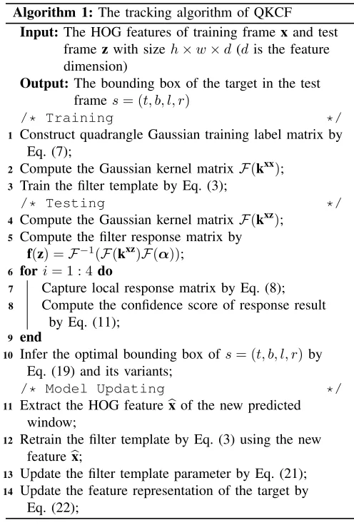
V. COMPLEXITYANALYSIS

Algorithm 1: The tracking algorithm of QKCF Input:The HOG features of training framex and test

framezwith size h×w×d(dis the feature dimension)

Output: The bounding box of the target in the test frames= (t, b, l, r)

/* Training */

1 Construct quadrangle Gaussian training label matrix by

Eq. (7);

2 Compute the Gaussian kernel matrix F(kxx); 3 Train the filter template by Eq. (3);

/* Testing */

4 Compute the Gaussian kernel matrix F(kxz);

5 Compute the filter response matrix by

f(z) =F−1_(F(kxz_)F(α)); 6 fori= 1 : 4do

7 Capture local response matrix by Eq. (8); 8 Compute the confidence score of response result

by Eq. (11);

9 end

10 Infer the optimal bounding box of s= (t, b, l, r)by

Eq. (19) and its variants;

/* Model Updating */

11 Extract the HOG feature_bxof the new predicted

window;

12 Retrain the filter template by Eq. (3) using the new

feature_bx;

13 Update the filter template parameter by Eq. (21); 14 Update the feature representation of the target by

Eq. (22);

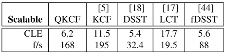
extra filters like part-based tracker. As in Algorithm 1, the whole process can be divided into 4 parts, including training, testing, inference and model updating. Approximately, in the phase of training and testing, the complexity of training should be the same as the original KCF [5]. In the inference phase, when calculating the exact coordinates of the target based on weighted Bayesian inference, our method brings in an extra cost ofO(s2), wheresis the side length of the local response matrix. Compared to the overall costs of training and testing, this extra cost is rather small and can be negligible. In the model updating phase, though our strategy is slightly different from KCF [5], calculating an extra weight parameter w as Eq. (20) specified has a cost of O(1). Therefore, QKCF is equivalent to KCF [5] in terms of the complexity. This is confirmed by the results reported in Table. IV, where the obtained FPSs (frames per second) of two algorithms are 168 and 195, respectively.

VI. EXPERIMENTS

To validate the effectiveness of the proposed QKCF method for visual tracking, we carry out extensive experiments in both scalable and unscalable situations with comparisons to state-of-the-art methods.

TABLE I

THE AVERAGE TRACKING PERFORMANCE COMPARISON OF THE PROPOSED

METHOD WITH STATE-OF-THE-ART METHODS ON THEOTB-100DATASET MEASURED BYCLEAND F/S.

OTB-100 QKCF KCF [5] DSST [18] LCT [17]

CLE 40.6 40.4 40.9 38.2

f/s 165.5 198 29.9 17.6

Fig. 5. Precision and success plots over the 100 video sequences in the OTB-100 dataset.

A. Datasets

For evaluation, we employ 100 video sequences in OTB-100, a large object tracking benchmark dataset [6], covering all difficult situations, such as illumination variation, scale variation, occlusion, background clutter and motion blur. To better compare the performance on scalable tracking, we select 16 sequences from OTB-100, where severe scale variations arise.

B. Experimental Settings

The proposed QKCF algorithm is implemented in Matlab and evaluated on a desktop with an Intel (R) Core (TM) i5-3470 3.20 GHz CPU and 8 GB RAM.

Fig. 6. Performance of different learning rateµon OTB-100.

estimated centre location of the target object, while the average distance precision is plotted over a range of thresholds in the precision plot. Following the PASCAL evaluation criteria [43], success plot is used to measure bounding box overlap rate. Finally, we provide the visualized qualitative analysis of our approach with comparison to existing tracking methods.

Baseline Methods. On the overall tracking in OTB-100, we tested 5 state-of-the-art trackers. They are KCF [5], SWCF [45], DSST [18], fDSST [44] and LCT [17], where the last three ones are scalable trackers. On the scalable dataset, we use 4 trackers of them as baseline which includes KCF [5], DSST [18], fDSST [44], LCT [17].

Implementation Details. Empirically, β in Eq. (20) is set to 1, while the learning rate µ in Eq. (21) is set to 0.03. As in [18], we use densely sampled HOG [46] for image representation. Using a cell size of 4×4, we can extract the features with length 992, which are always multiplied by a Hann window [7].

C. On the Overall Tracking in OTB-100

The average performance on CLE and the computational efficiency for the 100 video sequences tested on the OTB-100 dataset is shown in Table I, and its corresponding precision and success plot are shown in Figure 5. From Table I, we can find that the six trackers perform competitively for the unscalable tracking. It reveals that KCF [5] and its variants perform stably when tracking objects in most situations.

Seen from Figure 5, we can observe that the performance of QKCF is similar to that of KCF [5], and is higher than fDSST [44] and SWCF [45], while DSST [18] and LCT [17] perform better than the proposed QKCF and un-scalable KCF [5] on overlap precision in the OTB-100 dataset. However, the better performance of DSST [18] and LCT [17] comes with the great sacrifice of computational efficiency, which is confirmed by the fact that QKCF tracker is 5 to 10 times faster than DSST [18] and LCT [17]. The reason behind is that only one filtering operation is required for each frame in QKCF, while one 3D template based filtering and 33 2D template based filtering are operated on the default 33-layer spatial pyramid for DSST [18] and LCT [17], respectively.

Additionally, we also conduct sensitivity tests when varying parameter β in Eq. (20) and the learing rate µ in Eq. (21). Because the standard deviation of weights is so small in most

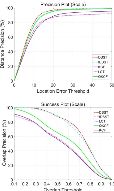
Fig. 7. Precision and success plots over the 16 video sequences with significant scale variations.

cases that the results are not that sensitive to β, which can be simply set to 1. As for the learning rateµ, the results are shown in Figure 6.

D. On Scalable Visual Tracking

The average performance of CLE and the computational efficiency for the 16 video sequences with significant scale variations is shown in Table IV, while the performance for each sequence is shown in Table II and Table III, respectively. The precision and success plot are shown in Figure 7.

We can find from Table II that the proposed QKCF method achieves the best performance in 3 of the 16 sequences on CLE, while DSST [18] , LCT [17] and fDSST [44] perform best on 5, 3, 4 sequences, respectively. Further, the CLE of QKCF is relatively stable without significant changes. KCF [5] is the most sensitive to scale variation, which indicates that KCF cannot well handle the scale variation. The results demonstrate the effectiveness and robustness of QKCF for scalable tracking.

From Table IV, it is clear that the tracking speed of QKCF is 5 to 8 times faster than DSST [18] and LCT [17] for scalable tracking. From Table III, we can find that the proposed QKCF method achieves the best performance in 4 of the 16 sequences on computational efficiency, while KCF [5] performs best on the other 12 sequences. Even on the challenging Car4

TABLE II

THE PERFORMANCE COMPARISON OF THE PROPOSED METHOD WITH STATE-OF-THE-ART METHODS ON SCALABLE VISUAL TRACKING MEASURED BY

CLE. THE BEST PERFORMANCES ARE HIGHLIGHTED BY BOLD.

Blur Car Cros Sing Sing Skat Sylve Twin Walk Walk

CLE Body Car1 Car2 Car24 Car4 Scale sing Dog1 er1 er2 ing1 ster Toy ings ing1 ing2 [44]QKCF 15.8 0.951 1.27 1.73 9.9 12.4 1.78 3.69 4.88 9.05 6.06 5.93 7.6 11.2 3.44 2.75

KCF [5] 17.5 42.4 3.97 4.1 9.88 16.1 2.25 4.39 12.8 10.3 7.67 5.1 7.8 6.77 3.97 29 DSST [18] 12.7 1.35 1.25 1.26 1.82 19.1 1.52 3.87 3.66 7.78 8.32 6.06 8.73 3.6 1.63 3.4 LCT [17] 7.86 134 2.65 9.07 6.60 25.1 2.03 3.28 7.23 7.55 6.21 4.82 9.2 11.8 3.04 42.7 fDSST [44] 6.12 1.22 1.41 4.39 1.72 9.91 1.51 2.69 3.69 7.78 7.58 6.56 9.42 12 2.07 12.2

TABLE III

THE EFFICIENCY COMPARISON OF THE PROPOSED METHOD WITH STATE-OF-THE-ART METHODS ON SCALABLE VISUAL TRACKING MEASURED BY F/S. THE HIGHEST EFFICIENCY IS HIGHLIGHTED BY BOLD.

Blur Car Cros Sing Sing Skat Sylve Twin Walk Walk

f/s Body Car1 Car2 Car24 Car4 Scale sing Dog1 er1 er2 ing1 ster Toy ings ing1 ing2

QKCF 87.1 141 155 290 63.8 264 303 188 118 148 152 157 123 133 217 147

KCF [5] 108 131 198 356 74.7 331 356 203 108 200 158 156 131 233 251 133 DSST [18] 3.75 27.8 29.9 41.4 10.2 46.6 64.3 63.2 4.22 29.8 25.8 30.6 20.9 53.6 42.8 25.0 LCT [17] 12.3 14.8 9.12 29.0 11.5 22.7 35.6 9.54 17.9 28.2 10.8 17.1 13.2 28.0 30.1 21.6 fDSST [44] 15.3 102 113 145 64.6 85.7 129 124 21 10.5 97.7 112 118 75.1 111 86.5

——QKCF ——KCF ——DSST ——LCT

Fig. 8. Tracking results of our QKCF algorithm, KCF [5], DSST [18] and LCT [17] methods on six challenging sequences (from top to bottom areCar1, Car24,Dog1,Human8,VolkswagenandWalking2, respectively).

LCT [17] can track the object with 30 f/s, which may not be used for real-time tracking. On the sequences with obvious shaking (beginning with Blur) and light and shadow changes (Car1), the tracking speeds of both DSST [18] and LCT [17] are below 20 f/s, while QKCF can process 120 f/s, which is robust to shaking and light and shadow changes. Compared with KCF [5], the efficiency of QKCF is slightly lower, which is caused by the weighted Bayesian inference in Section IV.

TABLE IV

THE AVERAGE EFFICIENCY COMPARISON OF THE PROPOSED METHOD WITH STATE-OF-THE-ART METHODS ON THE16SCALABLE SEQUENCES

MEASURED BY F/S.

[5] [18] [17] [44]

Scalable QKCF KCF DSST LCT fDSST

CLE 6.2 11.5 5.4 17.7 5.6

f/s 168 195 32.4 19.5 88

KCF is 6.92%. Therefore, we can conclude that the proposed QKCF significantly outperforms KCF on distance precision.

It is clear from the success plot that the proposed QKCF outperforms KCF [5] and LCT [17], but performs very slightly worse than DSST [18] and fDSST [44]. When setting the overlap threshold to 0.5, the overlap precision of QKCF is 64.8%, while the precisions of unscalable KCF [5], DSST [18], LCT [17] and fDSST [44] are 56.3%, 87.2%, 57.8% and 87.1%, respectively. The performance improvement of QKCF over KCF is 15.1%, from which we can again clearly view the superiority of QKCF over KCF.

To better show the tracking results with scale variations, we compare our algorithm with the other three state-of-the-art trackers (KCF [5], scalable DSST [18] and LCT [17]) on 6 challenging sequences, as shown in Figure 8.

From the above analysis, we can conclude that by sacrificing little computational efficiency, the proposed QKCF can signifi-cantly improve the distance precision and overlap precision for scalable tracking in a single frame single filter framework. The superior tracking precision and high computational efficiency make QKCF more practical than DSST [18] and LCT [17] for real-time tracking with significant scale variations.

E. Performance comparison of peak numbers

In principle, 2-peaks filter can already detect the location as well as the scale of object simultaneously. In this part of experiment, we intend to validate the effectiveness of 4-peaks strategy, compared to other numbers of peak. Therefore, apart from our QKCF (4-peaks filter) and the KCF (1-peak filter), we also include in the experiment two 2-peaks filters, one 3-peaks filter and one 5-3-peaks filter. Specifically, the first 2-3-peaks filter has positive samples in left-top and right-bottom corners (LT-RB for short) while the second 2-peaks filter has positive samples in LB-RT corners. Similarly, the 3-peaks filter has positive samples at LT-LB-RB corners, and the 5-peaks filter is a quadrangle filter plus a single peak in the center.

As for the estimation of the target window, we use a similar weighted Bayesian inference strategy. Specially, for 5-peaks filter we first use the same method to calculate the target window as quadrangle filter does, then adjust the location of the whole target window according to the additional center peak. Figure 9 depicts the obtained result.

Seen from the result, it is clear that the 4-peaks filter outperforms all the other peaks strategies. To be precise, two 2-peaks filters are far behind the 4-peaks filter; 5-peaks filter shows better precision than 2-peaks and 3-peaks strategies but is still slightly lower than 4-peaks filter in terms of the

Fig. 9. Precision and success plots over different numbers of peak.

performance. In general, more peaks lead to higher accuracy and better stability, because more information from various peaks is involved in estimating the bounding box of object. That interprets why 4-peaks filter looks much better than 2-peaks and 3-2-peaks filters. However, when we add an additional peak to the center, the precision gets lower on the contrary, which means the fifth peak is redundant and may provide useless information. The result turns out that choice of 4 peaks is a good trade-off between algorithm efficiency and accuracy.

VII. CONCLUSION ANDFUTUREWORK

label matrix to other applications, such as image retrieval [55]– [57], human action recognition [58], [59], and visual saliency detection [60], [61], is also worth studying.

REFERENCES

[1] A. Yilmaz, O. Javed, and M. Shah, “Object tracking: A survey,”ACM Computing Surveys, vol. 38, no. 4, p. 13, 2006.

[2] A. W. M. Smeulders, D. M. Chu, R. Cucchiara, S. Calderara, A. De-hghan, and M. Shah, “Visual tracking: An experimental survey,”IEEE Transactions on Pattern Analysis and Machine Intelligence, vol. 36, no. 7, pp. 1442–1468, 2014.

[3] H. Zhou, H. Kong, L. Wei, D. Creighton, and S. Nahavandi, “Efficient road detection and tracking for unmanned aerial vehicle,”IEEE Transac-tions on Intelligent Transportation Systems, vol. 16, no. 1, pp. 297–309, 2015.

[4] J.-P. Jodoin, G.-A. Bilodeau, and N. Saunier, “Tracking all road users at multimodal urban traffic intersections,”IEEE Transactions on Intelligent Transportation Systems, vol. 17, no. 11, pp. 3241–3251, 2016. [5] J. F. Henriques, R. Caseiro, P. Martins, and J. Batista, “High-speed

tracking with kernelized correlation filters,” IEEE Transactions on Pattern Analysis and Machine Intelligence, vol. 37, no. 3, pp. 583–596, 2015.

[6] Y. Wu, J. Lim, and M.-H. Yang, “Online object tracking: A benchmark,” in IEEE Conference on Computer Vision and Pattern Recognition (CVPR), 2013, pp. 2411–2418.

[7] D. S. Bolme, J. R. Beveridge, B. A. Draper, and Y. M. Lui, “Visual object tracking using adaptive correlation filters,” inIEEE Conference on Computer Vision and Pattern Recognition (CVPR), 2010, pp. 2544– 2550.

[8] J. F. Henriques, R. Caseiro, P. Martins, and J. Batista, “Exploiting the circulant structure of tracking-by-detection with kernels,” inEuropean conference on computer vision, 2012, pp. 702–715.

[9] M. Danelljan, F. Khan, M. Felsberg, and J. Weijer, “Adaptive color at-tributes for real-time visual tracking,” inIEEE Conference on Computer Vision and Pattern Recognition (CVPR), 2014, pp. 1090–1097. [10] K. Zhang, L. Zhang, Q. Liu, D. Zhang, and M.-H. Yang, “Fast visual

tracking via dense spatio-temporal context learning,” inEuropean Con-ference on Computer Vision (ECCV), 2014, pp. 127–141.

[11] S. Hare, A. Saffari, and P. H. Torr, “Struck: Structured output tracking with kernels,” in IEEE International Conference on Computer Vision (ICCV), 2011, pp. 263–270.

[12] Z. Kalal, K. Mikolajczyk, and J. Matas, “Tracking-learning-detection,” IEEE Transactions on Pattern Analysis and Machine Intelligence, vol. 34, no. 7, pp. 1409–1422, 2012.

[13] B. Babenko, M.-H. Yang, and S. Belongie, “Robust object tracking with online multiple instance learning,”IEEE Transactions on Pattern Analysis and Machine Intelligence, vol. 33, no. 8, pp. 1619–1632, 2011. [14] Y. Wu, B. Shen, and H. Ling, “Online robust image alignment via iterative convex optimization,” inIEEE Conference on Computer Vision and Pattern Recognition (CVPR), 2012, pp. 1808–1814.

[15] N. Dalal and B. Triggs, “Histograms of oriented gradients for human detection,” inIEEE Conference on Computer Vision and Pattern Recog-nition (CVPR), 2005, pp. 886–893.

[16] T. Liu, G. Wang, and Q. Yang, “Real-time part-based visual tracking via adaptive correlation filters,” inIEEE Conference on Computer Vision and Pattern Recognition (CVPR), 2015, pp. 4902–4912.

[17] C. Ma, X. Yang, C. Zhang, and M.-H. Yang, “Long-term correlation tracking,” inIEEE Conference on Computer Vision and Pattern Recog-nition (CVPR), 2015, pp. 5388–5396.

[18] M. Danelljan, G. Häger, F. Khan, and M. Felsberg, “Accurate scale esti-mation for robust visual tracking,” inBritish Machine Vision Conference (BMVC), 2014.

[19] S. Zhang, H. Yao, X. Sun, and X. Lu, “Sparse coding based visual tracking: Review and experimental comparison,”Pattern Recognition, vol. 46, no. 7, pp. 1772–1788, 2013.

[20] D. S. Bolme, B. A. Draper, and J. R. Beveridge, “Average of synthetic exact filters,” in IEEE Conference on Computer Vision and Pattern Recognition (CVPR), 2009, pp. 2105–2112.

[21] T. Lindeberg, “Scale selection properties of generalized scale-space interest point detectors,”Journal of Mathematical Imaging and vision, vol. 46, no. 2, pp. 177–210, 2013.

[22] Z. Kalal, J. Matas, and K. Mikolajczyk, “Pn learning: Bootstrapping binary classifiers by structural constraints,” in IEEE Conference on Computer Vision and Pattern Recognition (CVPR), 2010, pp. 49–56.

[23] M. Danelljan, A. Robinson, F. S. Khan, and M. Felsberg, “Beyond correlation filters: Learning continuous convolution operators for visual tracking,” inEuropean Conference on Computer Vision, 2016, pp. 472– 488.

[24] S. Hong, T. You, S. Kwak, and B. Han, “Online tracking by learning discriminative saliency map with convolutional neural network,” in International Conference on Machine Learning, 2015, pp. 597–606. [25] C. Ma, J.-B. Huang, X. Yang, and M.-H. Yang, “Hierarchical

con-volutional features for visual tracking,” in Proceedings of the IEEE International Conference on Computer Vision, 2015, pp. 3074–3082. [26] L. Wang, W. Ouyang, X. Wang, and H. Lu, “Visual tracking with

fully convolutional networks,” inProceedings of the IEEE International Conference on Computer Vision, 2015, pp. 3119–3127.

[27] H. Nam and B. Han, “Learning multi-domain convolutional neural networks for visual tracking,” in Proceedings of the IEEE Conference on Computer Vision and Pattern Recognition, 2016, pp. 4293–4302. [28] R. Tao, E. Gavves, and A. W. Smeulders, “Siamese instance search for

tracking,” inProceedings of the IEEE Conference on Computer Vision and Pattern Recognition, 2016, pp. 1420–1429.

[29] J. Sanchez-Riera, K. Srinivasan, K.-L. Hua, W.-H. Cheng, M. A. Hossain, and M. F. Alhamid, “Robust rgb-d hand tracking using deep learning priors,”IEEE Transactions on Circuits and Systems for Video Technology, 2017.

[30] S. Avidan, “Ensemble tracking,”IEEE transactions on Pattern Analysis and Machine Intelligence, vol. 29, no. 2, 2007.

[31] Q. Bai, Z. Wu, S. Sclaroff, M. Betke, and C. Monnier, “Randomized en-semble tracking,” inProceedings of the IEEE International Conference on Computer Vision, 2013, pp. 2040–2047.

[32] N. Wang and D.-Y. Yeung, “Ensemble-based tracking: Aggregating crowdsourced structured time series data.” inInternational Conference on Machine Learning (ICML), 2014, pp. 1107–1115.

[33] R. O. Chavez-Garcia and O. Aycard, “Multiple sensor fusion and clas-sification for moving object detection and tracking,”IEEE Transactions on Intelligent Transportation Systems, vol. 17, no. 2, pp. 525–534, 2016. [34] X. Sun, H. Yao, S. Zhang, and D. Li, “Non-rigid object contour tracking via a novel supervised level set model,” IEEE Transactions on Image Processing, vol. 24, no. 11, pp. 3386–3399, 2015.

[35] M. Demi, “Contour tracking with a spatio-temporal intensity moment,” IEEE transactions on Pattern Analysis and Machine Intelligence, vol. 38, no. 6, pp. 1141–1154, 2016.

[36] J. Fang, H. Xu, Q. Wang, and T. Wu, “Online hash tracking with spatio-temporal saliency auxiliary,”Computer Vision and Image Understand-ing, vol. 160, pp. 57–72, 2017.

[37] Q. Wang, J. Fang, and Y. Yuan, “Multi-cue based tracking,” Neurocom-puting, vol. 131, pp. 227–236, 2014.

[38] S.-H. Bae and K.-J. Yoon, “Robust online multi-object tracking based on tracklet confidence and online discriminative appearance learning,” in IEEE Conference on Computer Vision and Pattern Recognition (CVPR), 2014, pp. 1218–1225.

[39] A. Vatavu, R. Danescu, and S. Nedevschi, “Stereovision-based multiple object tracking in traffic scenarios using free-form obstacle delimiters and particle filters,” IEEE Transactions on Intelligent Transportation Systems, vol. 16, no. 1, pp. 498–511, 2015.

[40] L. Fagot-Bouquet, R. Audigier, Y. Dhome, and F. Lerasle, “Improving multi-frame data association with sparse representations for robust near-online multi-object tracking,” in European Conference on Computer Vision (ECCV). Springer, 2016, pp. 774–790.

[41] J. Hong Yoon, C.-R. Lee, M.-H. Yang, and K.-J. Yoon, “Online multi-object tracking via structural constraint event aggregation,” in IEEE Conference on Computer Vision and Pattern Recognition (CVPR), 2016, pp. 1392–1400.

[42] A. K. KC, L. Jacques, and C. De Vleeschouwer, “Discriminative and efficient label propagation on complementary graphs for multi-object tracking,” IEEE transactions on Pattern Analysis and Machine Intelligence, vol. 39, no. 1, pp. 61–74, 2017.

[43] M. Everingham, L. Van Gool, C. K. Williams, J. Winn, and A. Zisser-man, “The pascal visual object classes (voc) challenge,”International Journal of Computer Vision, vol. 88, no. 2, pp. 303–338, 2010. [44] M. Danelljan, G. Häger, F. S. Khan, and M. Felsberg, “Discriminative

scale space tracking,”IEEE transactions on pattern analysis and ma-chine intelligence, vol. 39, no. 8, pp. 1561–1575, 2017.

[45] E. Gundogdu and A. A. Alatan, “Spatial windowing for correlation filter based visual tracking,” inIEEE International Conference on Image Processing (ICIP), 2016, pp. 1684–1688.

IEEE Transactions on Pattern Analysis and Machine Intelligence, vol. 32, no. 9, pp. 1627–1645, 2010.

[47] J. Fan, W. Xu, Y. Wu, and Y. Gong, “Human tracking using convolu-tional neural networks,”IEEE Transactions on Neural Networks, vol. 21, no. 10, pp. 1610–1623, 2010.

[48] N. Wang and D.-Y. Yeung, “Learning a deep compact image representa-tion for visual tracking,” inAdvances in Neural Information Processing Systems (NIPS), 2013, pp. 809–817.

[49] S. Hong, T. You, S. Kwak, and B. Han, “Online tracking by learning discriminative saliency map with convolutional neural network.” in International Conference on Machine Learning (ICML), 2015, pp. 597– 606.

[50] Y. Qi, S. Zhang, L. Qin, H. Yao, Q. Huang, J. Lim, and M.-H. Yang, “Hedged deep tracking,” inProceedings of the IEEE Conference on Computer Vision and Pattern Recognition, 2016, pp. 4303–4311. [51] J. Gao, Q. Wang, and Y. Yuan, “Embedding structured contour and

loca-tion prior in siamesed fully convoluloca-tional networks for road detecloca-tion,” IEEE Transactions on Intelligent Transportation Systems, 2017. [52] Q. Wang, J. Gao, and Y. Yuan, “A joint convolutional neural networks

and context transfer for street scenes labeling,”IEEE Transactions on Intelligent Transportation Systems, 2017.

[53] Q. Wang, J. Wan, and Y. Yuan, “Deep metric learning for crowdedness regression,” IEEE Transactions on Circuits and Systems for Video Technology, 2017.

[54] S. Zhao, H. Yao, Y. Gao, R. Ji, and G. Ding, “Continuous probability distribution prediction of image emotions via multitask shared sparse regression,”IEEE Transactions on Multimedia, vol. 19, no. 3, pp. 632– 645, 2017.

[55] Y. Guo, G. Ding, L. Liu, J. Han, and L. Shao, “Learning to hash with optimized anchor embedding for scalable retrieval,”IEEE Transactions on Image Processing, vol. 26, no. 3, pp. 1344–1354, 2017.

[56] Z. Lin, G. Ding, J. Han, and J. Wang, “Cross-view retrieval via probability-based semantics-preserving hashing,”IEEE Transactions on Cybernetics, vol. 47, no. 12, pp. 4342–4355, 2017.

[57] Y. Guo, G. Ding, J. Han, and Y. Gao, “Zero-shot learning with transferred samples,”IEEE Transactions on Image Processing, vol. 26, no. 7, pp. 3277–3290, 2017.

[58] B. Zhang, A. Perina, Z. Li, V. Murino, J. Liu, and R. Ji, “Bounding multiple gaussians uncertainty with application to object tracking,” International Journal of Computer Vision, vol. 118, no. 3, pp. 364–379, 2016.

[59] B. Zhang, Y. Yang, C. Chen, L. Yang, J. Han, and L. Shao, “Action recognition using 3d histograms of texture and a multi-class boosting,” IEEE Transactions on Image Processing, vol. 26, no. 10, pp. 4648–4660, 2017.

[60] D. Zhang, J. Han, L. Jiang, S. Ye, and X. Chang, “Revealing event saliency in unconstrained video collection,”IEEE Transactions on Image Processing, vol. 26, no. 4, pp. 1746–1758, 2017.

[61] X. Yao, J. Han, D. Zhang, and F. Nie, “Revisiting co-saliency detection: a novel approach based on two-stage multi-view spectral rotation co-clustering„”IEEE Transactions on Image Processing, vol. 26, no. 7, pp. 3196–3209, 2017.

Guiguang Dingreceived the Ph.D. degree in elec-tronic engineering from Xidian University, China. He is currently an Associate Professor with the School of Software, Tsinghua University. Since 2006, he has been a postdoctoral research fellow with the Department of Automation, Tsinghua Uni-versity. His current research centers on the area of multimedia information retrieval, computer vision, and machine learning.

Wenshuo Chenreceived her BS degree from School of Software, Nanjing University, Jiangsu, China in 2013, and currently is a MS candidate in School of Software in Tsinghua University, Beijing, China. Her research interests include multimedia information retrieval, human action recognition and video event detection.

Sicheng Zhao received the Ph.D. degree from Harbin Institute of Technology in 2016. He is now a postdoctoral research fellow in the School of Software, Tsinghua University, China. His research interests include affective computing, social media analysis and multimedia information retrieval.

Jungong Hanis a tenured faculty member with the School of Computing and Communications at Lan-caster University, LanLan-caster, UK. Previously, he was a faculty member with the Department of Computer and Information Sciences at Northumbria University, UK. His research interests include computer vision, image processing, machine learning, and artificial intelligence.