A Study on Handling Non Linear Separation of Classes
using Kernel based Supervised Noise Clustering
Approach
Ishuita SenGupta
College of Computing Sciencesand Information Technology Teerthanker Mahaveer University
Moradabad, India
Anil Kumar,
PhD Photogrammetry & RemoteSensing Department Indian Institute of Remote Sensing
Dehradun, India
Rakesh Kumar Dwivedi,
PhD College of Computing Sciencesand Information Technology Teerthanker Mahaveer University
Moradabad, India
ABSTRACT
This paper presents a framework of incorporating kernel methods with fuzzy based image classifiers. The goal of image classification is to separate images according to their visual content into two or more disjoint classes. The work demonstrates how non linearity among the different classes of remote sensing data with uncertainty are handled with Noise classifier without entropy(fuzzy classifier) using kernel approach for land use/land cover maps generation. It also show case the comparative study between performance of Noise Classifier with Euclidean Distance and Noise Classifier with Kernel functions. The introduction to Kernel function in fuzzy based classification techniques provides the basis for the development of more robust approaches to the classification problem.
Keywords
Image Classification, Fuzzy Classifier, Kernel functions.
1.
INTRODUCTION
Fuzzy Classifiers are based on the idea of fuzzy set logic by introducing degree of vagueness or fuzziness with membership function. According to the concept a pixel or a sample can be assigned to more than one class with the grade of membership value ranging between 0 and 1[1,2]. The value nearer to 1 resembles higher membership of the sample or pixel to the class [3,4]. It is perceived that fuzzy based information can become complete by adding entropy to the standard one, since it can observe the nature of both methods more deeply by contrasting these two methods (Dunn, 1974 and Bezdek ,1984).Studies and related implementations have been done by connecting entropy with standard fuzzy based techniques[5].
Primary motivations is to hybridize fuzzy based classifier with entropy for the purpose of optimization with respect to membership values and cluster centers and that the constraint is same for both where, the difference between two methods is the use of an objective function[6,7].
Present Paper discusses the effect of incorporating Kernel functions with supervised Noise Clustering with Entropy. The upcoming section portrays the role of Kernel functions and their study.
2.
KERNEL FUNCTIONS
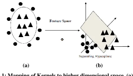
Fuzzy based classifiers are effective on the data by linear boundaries, and in order to extend classifier functionality to classify by non-linear boundaries the kernel functions are used [8]. A kernel function maps data from original input feature space to a higher dimensional feature space where the
problem of nonlinearity can be resolved (Illustrated in Fig 1).
[image:1.595.328.541.262.384.2](a) (b)
Fig 1: Mapping of Kernels to higher dimensional space. (a) Non-linearly separable data in input feature space (b) Linearly separated data in transformed kernel feature
space
The kernel method adds capability to linear algorithms to separate the non-linearly separable classes. The kernel method projects the data from the input feature space to higher dimensional feature space [10]. Each coordinate in the input feature space corresponds to one feature. In this higher dimensional feature space, the non-linearly separable classes may appear to be linearly separable or better structured. The aim of kernel method is to identify a linearly separating hyperplane that separates the classes Figure 1in higher dimensional feature space [13]. As depicted from Figure 1 (a), the data available was not linearly separable in two dimensional feature space. In Figure 1(b), the data when mapped to a three (higher) dimensional feature space becomes linearly separable by a hyperplane. The features are the attribute that adds uniqueness to the feature vector, so that they can be uniquely identified. All kernel methods used in this research work are either dot product function, e.g. global kernels or distance function e.g. local kernels.
In equation (2.1) the feature map ( ) is the mapping function that non-linearly maps the data to a higher dimensional feature space. For example, in equation (2.2) the kernel function ( ) implicitly computes the dot product between two vectors and i in higher dimensional feature space without
explicitly transforming and i to that higher dimensional feature space, this technique is known as “Kernel trick”[9].
q p
R
R
:
, where p<q (2.1)K(
i
x
x
,
)=
x
.
x
i (2.2)The kernel method projects the data from the input feature space to higher dimensional feature space. All kernel methods used in this research work are either dot product function, e.g. global kernels or distance function e.g. local kernels.
2.2.1 Local Kernels
They are based on evaluation of the quadratic distance between training samples and the mean vector of the class. Only feature vectors that are close or in proximity of each other have an influence on the kernel value. In this research, the value of the input vector was normalized between [0, 1] and thus acceptable result can be produced at " " equals 1. The different local kernels were defined as follows:
Radial basis function (RBF) kernel
The RBF kernel is defined by exponential function as shown in equation (2.3). Here, i is the feature vector in the data and
is the mean vector of class . determines the width of the kernel; and are the constants. By replacing and by 1 the Gaussian kernel can be obtained. In this study the value of
and were taken to be 2 and 3 respectively [10, 12].
0 b a, σ, where , 2 2 2 ,
b j v a i x e j v i xK (2.3)
KMOD- (kernel with moderate decreasing)
KMOD is the distance based kernel function introduced by Ayat et. al.[8] as shown in equation (2.4). It shows better result in classifying closely related datasets (highly correlated) and has shown better accuracy than Radial Basis Function (RBF) and polynomial kernel.
0 , where , 1 2 2 ,
-j v i x e j v i xK (2.4)
The parameter and controls the decreasing speed of the kernel function and the width of the kernel respectively. In this study the value of was taken to be one.
Gaussian kernel
The Gaussian kernel is a special case of radial basis function kernel [11], shown in equation (2.5). Here, is the feature vector in the image and is the mean vector of the class.
0 where , 2 2 2 ,
b j v a i x e j v i xK (2.5)
Inverse Multi-quadratic (IMQ) kernel
The inverse multi-quadratic kernel is defined as in equation (2.6) [9,13]. Here the value of was taken to be one.
0 c where , 2 1 , c j v i x j v i x
K (2.6)
2.2.2 Global Kernels
In global kernels, the samples that are far away from each other have an influence on the kernel value. All the kernels which are based on the dot-product are global [13]. The different global kernels are as follows:
Linear kernel
Linear kernel is one of the simplest kernel functions. It is defined as the inner product of the input feature vectors, as shown in equation (2.7).
j i j
i
v
x
v
x
K
,
.
(2.7) Polynomial kernelThe polynomial kernel is a positive definite kernel i.e. each element of the kernel matrix (a kernel matrix is a × matrix of feature vector) is positive, shown in equation (2.8). defines the degree of the polynomial function and c is the constant [10]. In this work value of P has been taken from 1 to 4. The value of c has been taken to be zero.
.
,
where
c
0
,
P j i ji
v
x
v
c
x
K
(2.8)Sigmoid kernel
Sigmoid kernel is a hyperbolic tangent function, as shown in equation (2.9). The parameter work as scaling parameter for the kernel function and defines width of the kernel. The best possible value for and c were when > 0and c< 0 [11].
x
v
c
v
x
K
i j
i j
.
.
tanh
,
(2.9)2.2.3 Spectral Kernel
The spectral kernel takes into consideration the spectral signature concept [11], as shown in equation (2.10). These kernels are based on the use of spectral angle ( ,) to measures the distance between the feature vector and the mean vector of the class i. It is expressed as follows:
i i iv
x
v
x
v
x
,
arccos
.
(2.10)2.2.4 Hypertangent Kernel
The hyper tangent kernel is a hyperbolic tangent function, as shown in equation (2.11). The adjustable parameter defines the width or the scale of the kernel. Here and are the feature vectors in the data. It has been seen that the hyper tangent kernel outperforms other kernels when applied to a large data set [8, 12].
2 2| |
| |
tanh
1
,
i ix
x
K
(2.11)3.
STUDY AREA AND DATASET USED
study work is situated in Haridwar district in the state of Uttarakhand, India. Area extends from 29°52’49” N to 29°54’2” N and 78°9’43” E to 78°11’25” E. The site is identified with five land cover classes (Fig 2) i.e. Water, Wheat, Forest, Riverine Sand, Fallow Land. The reasons for selecting this study area include:
Landsat-8 and Formosat-2 images are available for selected site.
[image:3.595.56.280.206.416.2] Ground truth information is available and has been identified on six classes for Landsat-8 and Formosat-2 images.
Fig 2: Location of area under study
4.
ADOPTED METHODOLOGY
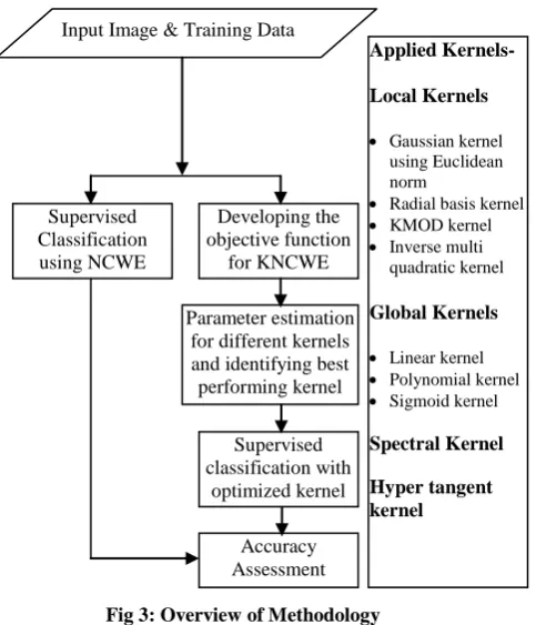
This section defines the methodology that has been adopted in order to achieve the desired objective. The overview of methodology has been represented in Fig 3.
Fig 3: Overview of Methodology
All steps mentioned above in Fig 3 – are briefly explained
below –
a) Input Image and the training data
Initially, the images of Formosat2 and Landsat8 were geometrically rectified and geo-registered. The training data or signature files for each class (water, wheat, forest, riverine sand and fallow land) has been taken from simulated FORMOSAT-2 image.
b) Developing the objective function for KNCWE
The Kernel based NC with Entropy classifier was formed by replacing the Euclidean distance norm present in the Noise classifier with kernel metric. Furthermore on simulated image the kernel based noise classifier algorithm as well as noise classifier with Euclidean distance has been applied.
c) Parameter estimation for different kernels and identifying best performing kernel
The parameter estimation is one of the most important steps in the classification process. Choosing the optimal parameter guarantees the best results from the classifier. Here, the developed KNCWE classifier has been implemented upon FORMOSAT 2 simulated image for different values of fuzzy parameter ranging between [1.1, 5.0] and the resolution parameter δ has been taken in the range of 1 to 106.
,the regularizing parameter ν has been considered from 0.01 to 106.
d) Supervised classification with optimized kernel
The supervised KNCWE classifier has been developed with an aim to handle non-linearity between the classes. In this step, the best kernel function selected from nine different kernel functions has been incorporated into Noise Classifier. The optimized valued parameters have been used for classification.
e) Accuracy Assessment
In this research work, a new method for evaluating the accuracy of classification was proposed. This method is known as simulated image technique. It has been used to estimate the results from NCWE and KNCWE classifier. As, the pixel composition is known in the simulated image so the results from the classifier can easily be verified. Also FERM (Fuzzy Error Matrix) method has been studied to strengthen the findings of simulated image technique. It is a modification of traditional error matrix for accuracy assessment of the soft classifier [14].
5.
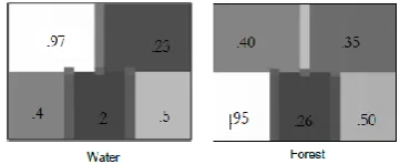
SIMULATED IMAGE TECHNIQUE
This underlying concept of this technique is assigning the fuzzy membership values to feature vectors based on the distance measure from the mean vector of the classes (mean vector). The simulated image is generated based on the sample data for each class with desired number of bands. With the simulated image, it is easy to compare the outcome of the classifier with the expected known input at a particular location. Also, it makes easy to identify the behavior of classifier with the mixed pixels. The mixed pixels can be simulated with varying proportions of different classes. Simulated image of multi-spectral data of Formosat-2 (4 bands) has been taken to study the performances of all the Kernels. In this simulated image, we have intentionally mixed classes in a specific ratio and also have created an intra-class variation. Based on these controlled conditions the ability of handling the mixed pixel problem and detecting the intra-class pixel value variation were tested on the simulated image. Input Image & Training Data
Supervised Classification using NCWE
Developing the objective function
for KNCWE
Parameter estimation for different kernels and identifying best performing kernel
Supervised classification with
optimized kernel
Accuracy Assessment
Applied Kernels-
Local Kernels
Gaussian kernel using Euclidean norm
Radial basis kernel
KMOD kernel
Inverse multi quadratic kernel
Global Kernels
Linear kernel
Polynomial kernel
Sigmoid kernel
Spectral Kernel
[image:3.595.57.299.471.753.2]Fig 4: Simulated Image of Formosat 2 (Class Distribution)
[image:4.595.77.258.301.375.2]The mixed pixels can be simulated with varying proportions of different classes. As shown in Fig 5, that simulated image is classified into fractional images by using soft classifier. The proportion of these classes in each individual fractional image can be identified and compared with the input. The membership value for a class in fractional image is affected by the distance criteria used for classification.
Fig 5: Simulated Image Class Output
6.
KERNEL BASED NOISE
CLUSTERING WITH ENTROPY
(KNCWE)
The KNCWE classifier is formed by using kernel methods with supervised Noise Clustering with entropy. It is expected to handle non-linearity in the data by implementation of kernel methods. The objective function of Noise classifier without entropy is mentioned below:
)
,
(
U
V
J
NCWE =
1 1 1 1 1 , 1 1 log , C i Nj ij ij m N c i j i N i C j m
ij D x v u u u
u (6.1)
C is the number of classes, N is the total number of pixels in the image, m is the fuzzification factor,
u
ijrepresent the membership value of ith pixel in the jth class,u
i,c1represents the membership values of the noise class,
v
j is the mean value (cluster center) of the jth class,x
i is the vector value of the ith pixel, D is the Euclidean distance between i x and j
v
and δ is a positive constant called the Noise distance,
is the regularizing parameter and has a value greater than 0.In KNC the kernel metric is used to compute distance between the cluster prototype (the mean value of the cluster) and the feature vector (pixel).This distance can be calculated in kernel higher dimension feature space without actual transformation of the feature vector to that higher dimensional feature space. The distance between two vectors in higher dimensional feature space can be expressed as:
k i ik
v
x
v
x
D
,
(6.2)In the higher dimensional feature space, the KNC objective function and the membership function μij can be expressed as
in equation (6.2) and (6.3) respectively.
The objective function for Kernel Based Noise Classifier (KNC) is derived as:
n m
k c k c i i k m n k
ki
x
v
u
u
1 1 , 1 1KNC
U,
V
J
(6.3) Computation of Membership Values:
c
i
v
x
v
x
v
x
u
c j m i k m j k i kij
,
1
1 1 1 1 2 1 2
(6.4) Where
c : Number of clusters n : Number of data points
xik : membership value of xk in class I
C : Number of classes m : Weighing component V: set of cluster centers
: Implicit non-linear map
δ: is a positive constant called the Noise distance(Resolution Parameter)
: Regularizing Parameter
x
v
i
c
u
c j m i k ck
1
,
1
1 1 1 2 1 ,
(6.5) Instead of Euclidean Distance as shown in equation (6.1) the mapping function in KNCWE is been replaced by kernel function as:
k i
k i
i
k
v
x
v
K
x
v
x
D
,
,
(6.6)Thus, KNCWE objective function has been generated by replacing the Euclidean distance metric by kernel distance metric in the NC objective function.
7.
RESULT AND ANALYSIS
7.1 Identifying the best kernel and
estimating the parameter
of 1.1, resolution parameter δ has been fixed to 10000,using these two fixed parameters KNCWE has been performed upon varying ν from 0.01 to 106
,resulting to optimized value at ν=100.
Sigmoid kernel following with Spectral kernel has been found to be best performing. Furthermore, Sigmoid based NCWE i.e. KNCWE classification was performed on Formosat-2 data as well on Landsat8 data.
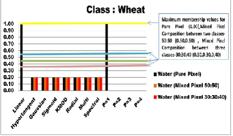
[image:5.595.314.543.89.408.2]Class composition at different pixel values of 9 different kernels have been computed analyzed using Formosat2 simulated image. Fig 6 shows the histogram of wheat class depicting the membership values corresponding to different ν. For the optimal classification, the membership value of pure pixel in the classified output of a class must be maximized. The mixed pixels were simulated with two variations, one with composition of 50:50 (shown as Mixed Pixel (50:50) and second between two different classes and other with composition of 30:30:40 The target membership are highlighted with yellow, purple and blue lines for the value expected from the pixel with full belongingness to a class must be close to 1, the target membership value of 0.50, 0.40 and 0.30 is expected from the pixel with 50%, 40% and 30% belongingness for a class respectively.
Fig 6: Graphical Representation of various Kernels with respect to membership values.
8.
ACCURACY ASSESSMENT
8.1 Accuracy Assessment of Single Kernels
Apart from image to image accuracy assessment , simulated image method has been used to depict the variations on class wise membership values as shown in Figure 6.FERM(Fuzzy Error Matrix),SCM (Sub-Pixel Confusion Uncertainty Matrix), MIN PROD, MIN MIN, MIN LEAST techniques have been applied for fractional output variation. Table 1(a) and 1(b) shows the overall accuracy computed of all the kernels, and the statistics demonstrates that Sigmoid and Spectral kernels have shown the highest accuracy among all. Fig 7 represents an overall accuracy histogram of individual kernel corresponding to varying m (Fuzzifier).Table 2 demonstrates the class wise accuracy including both user and producer accuracy as well as overall accuracy of Sigmoid based Noise Classifier. Plotting of overall accuracy corresponding to various accuracy assessment techniques is shown in Fig 8. It also depicts that the optimized regularizing parameter
has been found to be 100.Table 1(a): Tabular representation of overall accuracy using FERM of individual Kernels
Kernels→ ν
↓ Linear P1 P2 P3 P4
Hyper tangent
0.01 0.00% 0.00% 0.00% 0.00% 0.00% 73.17% 0.02 0.00% 0.00% 0.00% 0.00% 0.00% 73.04% 0.05 0.00% 0.00% 0.00% 0.00% 0.00% 65.37%
0.08 0.00% 0.00% 0.00% 0.00% 0.00% 62.24% 0.1 0.00% 0.00% 0.00% 0.00% 0.00% 60.15% 0.2 0.00% 0.00% 0.00% 0.00% 0.00% 59.66% 0.5 0.00% 0.00% 0.00% 0.00% 0.00% 71.78%
0.8 0.00% 0.00% 0.00% 0.00% 0.00% 80.63% 1 0.00% 0.00% 0.00% 0.00% 0.00% 84.20% 5 0.00% 0.00% 0.00% 0.00% 0.00% 96.80% 10 0.00% 0.42% 0.00% 0.00% 0.00% 98.41%
100 0.21% 0.00% 0.00% 0.00% 0.00% 99.66% 1000 0.21% 0.33% 0.00% 0.00% 0.00% 99.68% 10000 0.07% 0.28% 0.00% 0.00% 0.00% 100.0%
100000 1.26% 0.00% 0.00% 0.00% 0.00% 100.0% 1000000 7.53% 7.56% 0.00% 0.00% 0.00% 100.0% *P1 – Polynomial (Degree 1), P2 – Polynomial (Degree 2), P3 – Polynomial (Degree 3), P4 – Polynomial (Degree 4)
Table 1 (b): The tabular representation of overall accuracy using FERM for Single Kernels
Kernels → ν ↓
Gaussia
n Radial KMOD Multi quadrat ic
Sigmoi d
Spectr al
0.01 70.71% 72.14% 73.15% 72.65% 55.91% 74.31% 0.02 67.63% 72.85% 74.93% 66.49% 54.15% 74.24%
0.05 59.59% 65.07% 70.85% 58.08% 63.18% 75.38% 0.08 57.77% 59.73% 70.41% 60.03% 72.79% 76.71% 0.1 58.43% 57.90% 67.21% 61.52% 76.16% 78.17%
0.2 67.42% 60.80% 61.89% 72.09% 86.55% 83.33% 0.5 81.05% 75.33% 67.63% 85.99% 94.30% 91.03% 0.8 86.48% 82.58% 75.41% 90.59% 96.41% 94.21% 1 88.49% 85.74% 79.84% 92.44% 96.99% 94.98%
5 97.33% 96.98% 95.82% 98.35% 99.29% 98.92% 10 98.66% 98.44% 98.03% 99.14% 99.60% 99.46% 100 99.80% 99.70% 99.65% 99.75% 99.63% 99.80%
[image:5.595.55.283.331.464.2]Histogram in Fig 7 shows that Sigmoid followed by Spectral are best performing kernel, showing highest accuracy.
Fig 7: Histogram of the overall accuracy using Fuzzy Error Matrix technique of different kernels
Table 2 shows the user and producer accuracy for every class. The kernel considered is Sigmoid with optimum value of regularizing parameter as 100.
Table 2. FERM based accuracy assessment for classified result of Landsat-8 dataset using Sigmoid Kernel based Noise Clustering Classifier
Class-wise Accuracy FERM Percentage
Water
User Accuracy 97.70%
Producer Accuracy 94.74%
Wheat
User Accuracy 92.02%
Producer Accuracy 95.89%
Forest
User Accuracy 94.22%
Producer Accuracy 96.57%
Riverine Sand
User Accuracy 96.00%
Producer Accuracy 96.57%
Fallow Land
User Accuracy 97.93%
Producer Accuracy 93.92%
Average User Accuracy 95.57% Average Producer Accuracy 95.54%
Overall Accuracy 95.55%
[image:6.595.54.297.94.276.2]Fig 8: Overall Accuracy of Sigmoid Kernel using FERM, SCM, MIN-MIN, MIN-PROD, MIN-LEAST
Table 3. Image to Image based accuracy assessment for classified result of Landsat-8 dataset using Sigmoid kernel based Noise Clustering Classifier
Kernels→ν↓ FERM SCM MIN PROD
MIN MIN
MIN LEAST
0.01 55.91%
56.36%+-1.7% 56.17% 54.66% 58.06%
0.02 54.15%
55.12%+-4.66% 54.52% 50.46% 59.77%
0.05 63.18%
65.6%+-10.4% 63.79% 55.20% 76.01%
0.08 72.79%
75.31%+-11.54% 73.48% 63.77% 86.85%
0.1 76.16%
78.38%+-10.66% 76.89% 67.72% 89.03%
0.2 86.55%
88%+-7.78% 87.33% 80.22% 95.78%
0.5 94.30%
95.18%+-3.82% 95.08% 91.37% 99.00%
0.8 96.41%
97.08%+-2.64% 97.15% 94.45% 99.72%
1 96.99%
97.62%+-2.2% 97.72% 95.42% 99.82%
5 99.29%
99.62%+-0.38% 99.77% 99.24% 100.0%
10 99.60%
99.89%+-0.11% 99.94% 99.78% 100.0%
100 99.63%
99.9%+-0.1% 99.94% 99.80% 100.0%
1000 99.70%
99.88%+-0.12% 99.94% 99.76% 100.0% 10000 100.0% 100.00% 100.0% 100.0% 100.0%
100000 100.0% 100.00% 100.0% 100.0% 100.0% 1000000 100.0% 100.00% 100.0% 100.0% 100.0%
9.
MAJOR FINDINGS
[image:6.595.310.545.274.718.2] [image:6.595.48.287.359.679.2]Java developed application.
2) Computation of membership values has been done with a Java implemented utility, Band Membership Value Calculator.
3) Optimizing resolution parameter (δ), values taken, ranges from 10 to 106, and optimal value saturated at δ=10000. 4) Optimizing fuzzy parameter (m), values taken, ranges
from 1.1 to 5.5. It has been observed that the variation in m has not affected the variation in membership values throughout every kernel. Therefore, the optimized value of m has been fixed to 1.1.
5) Regularizing Parameter (ν) ranges from 0.01 to 106 has been considered to compute classified output by fixing other two parameters fixed=1.1 and δ=10000. Interval considered is 0.01 for this parameter and classification has been implemented for the defined range. Resulting to ν=100 as optimum value as shown in Fig 7.
6) The implementation of KNCWE algorithm has been accomplished by developing a tool. The class wise membership values shown in Fig 6 are near to zero of Polynomial Kernel with higher degree (p=2, 3, 4). The digital computation by the tool is completely integer based therefore the membership value of weaker performing kernels found to be fractional i.e. near to zero. The accuracy assessment as mentioned in Table 1(a) is also less in comparison to other kernels.
7) Similar traits have been shown in Linear and Polynomial Kernel with degree 1.In case of pure pixel they have performed well but failed in identification of mixed pixel composition, shown in Fig 6.
8) Implementing the KNCWE algorithm the two best kernels are found i.e. Sigmoid and Spectral. Table 2 shows that the highest accuracy has been found with Sigmoid Kernel followed by Spectral Kernel.
10.
CONCLUSION
According to the study of handling non linearity using kernel methods with fuzzy based classifier, this paper integrates the 9 kernels with noise classifier with entropy. It also highlights the effects of incorporating kernel methods, finding the best performing kernel.
The discussed kernels have shown better performance and have proven that fusing kernel methods with traditional classifier can output to upgrades in performance of classification. Behaviour of parameter optimization differs from kernel to kernel. Therefore, the parameter optimization for every kernel studied has been stabilized to a single value. Future work in the study is to perform a concrete analysis between traditional classifier Noise Clustering with Entropy and Kernel based Noise Clustering with Entropy Classifier.
11.
REFERENCES
[1] Zadeh, L. A. (1978). Fuzzy sets as a basis for a theory of possibility. Fuzzy Sets and Systems, 100, 9–34. http://doi.org/10.1016/S0165-0114(99)80004-9
[2] Bezdek, J. C., Ehrlich, R., and Full, W. (1984). FCM:
The fuzzy c-means clustering algorithm. Computers and
Geosciences, 10(2–3), 191–203.
http://doi.org/10.1016/0098-3004(84)90020-7
[3] Foody, G. M. (2000). Estimation of sub-pixel land cover composition in the presence of untrained classes. Computers and Geosciences, 26(4), 469–478. http://doi.org/10.1016/S0098-3004(99)00125-9 . [4] Upadhyay, P., Ghosh, S. K., and Kumar, A. (2014). A
Brief Review of Fuzzy Soft Classification and Assessment of Accuracy Methods for Identification of Single Land Cover. Studies in Surveying and Mapping Science (SSMS), 2(Mlc), 1–13.
[5] DAVÉ, R. & SEN, S. Noise clustering algorithm revisited. Fuzzy Information Processing Society, 1997. NAFIPS'97., 1997 Annual Meeting of the North American, 1997. IEEE, 199-204.
[6] Scholkopf, B., Burges, J. C., and Smola, A. J. (2008). Advances in Kernel Methods: Support Vector Learning, 373.
http://doi.org/10.1016/j.neuropsychologia.2011.01.001. [7] Dwivedi, R.K., Ghosh, S. K. and Kumar, A., 2013.
Visualization of Uncertainty using entropy on Noise clustering with entropy classifier. 3rd IEEE International Advance Computing Conference (IACC-2013).
[8] Byju, A. P. (2015). Non-Linear Separation of classes using a Kernel based Fuzzy c -Means ( KFCM ) Approach. ITC, University of twente,The Netherlands. [9] CHOTIWATTANA, W. Noise Clustering Algorithm
based on Kernel Method. Advance Computing Conference, 2009. IACC 2009. IEEE International, 2009. IEEE, 56-60.
[10] Hofmann, T., Scholkopf, B., and Smola, A. J. (2008). Kernel methods in machine learning. The Annals of
Statistics, 36(3), 1171–1220.
http://doi.org/10.1214/009053607000000677
[11] Lin, H., and Lin, C. (n.d.). A Study on Sigmoid Kernels for SVM and the Training of non-PSD Kernels by SMO-type Methods, 1–32.
[12] Mittal, D., and Tripathy, B. K. (2015). Efficiency Analysis of Kernel Functions In Uncertainty Based C-Means Algorithms. 2015 International Conference on Advances in Computing, Communications and Informatics (ICACCI), 807–813.
[13] Binaghi, E., Brivio, P. a., Ghezzi, P., and Rampini, A. (1999). A fuzzy set-based accuracy assessment of soft classification. Pattern Recognition Letters, 20(9), 935– 948. http://doi.org/10.1016/S0167-8655(99)00061-6 [14] USGS, Landsat Misson, Landsat8 Data Documentation
and Information, https://landsat.usgs.gov/landsat-8 [15] Formosat-2 eoPortal Directory, Formosat-2 Overview
and Specifications,