A Comprehensive Performance Analysis of GLCM DWT based Classification on Fingerprint Identification

(1)

A Comprehensive Performance Analysis of

GLCM-DWT-based Classification on Fingerprint Identification

Taner Çevik

Istanbul Aydin University

Istanbul, Turkey

Ali Mustafa Ali Alshaykha

Istanbul, Turkey

Nazife Çevik

Istanbul Arel University

Istanbul, Turkey

ABSTRACT

Fingerprint detection is one of the primary methods for identifying individuals. Gray Level Co-occurrence Matrix (GLCM) is the oldest and prominent statistical textual feature extraction method applied in many fields for texture analysis. GLCM holds the distribution of co-occurring intensity patterns at a given offset over a given image. However, images occupy excessive space in storage by its original sizes. Thus, Discrete Wavelet Transform (DWT) based compression has become popular especially for reducing the size of the fingerprint images. It is important to investigate whether GLCM-based classification can be utilized efficiently on DWT-compressed fingerprint images. In this paper, we analyze the performance of GLCM-based classification on DWT-compressed fingerprint images. We performed satisfying simulations for different levels of DWT-compressed images. Simulation results identify that classification performance sharply decreases by the increase of DWT-compression level. Besides, instead of utilizing all Haralick features, it is recognized that eight of them are the most prominent ones that affect the accuracy performance of the classification.

General Terms

Image Processing, Data Mining, Pattern Recognition.

Keywords

Fingerprint Detection, GLCM, DWT, Classification.

1. INTRODUCTION

Biometrics refers to the human specific behavioral and physiological characteristics belonging to a person which are distinctive of the other individuals and used for the personal identification [1-2]. A biometric system includes many distinctive personal biological characteristics such as iris, fingerprint, voice, signature or face recognition that are utilized for personal identification. Since biological features are unique and thus more reliable than traditional methods during individual identification, such systems are more useful and suitable than conventional procedures.

Biometric systems are now commonly used in different parts of everyday life such as building access and computer login. Fingerprint detection is one of the most prevalent methods for

personal identification within all biometric systems [3]. Throughout the world, fingerprint recognition is accepted by a large part of the population because of its fast, secure, and easy way of personal identification.

Fingerprints are the inherent parts of humans and unique for each individual. Even twins have different fingerprints. Using the patterns found on the finger tips, fingerprint biometric data is captured. As with every technology, using fingerprint for biometrics has its own advantages and disadvantages. Age of the user, dryness and wetness of the finger, temporary or permanent cuts on the finger, or dirt on the fingerprint scanner all cause the fingerprints to have weak patterns of ridge and valleys that can degrade the performance of a fingerprint biometric system. The mentioned issues lead to poor recognition rates in fingerprint identification system and users would have trouble with the system’s authentication process. Furthermore, as discussed before there can be artificial fingers, which threaten system’s security. For creating artificial fingers, a copy of the real fingerprint is required which can be obtained when the victim is touching objects like glasses and can be replicated in gelatin. For making the systems secure against artificial fingers, liveliness detection can be used. Liveliness detection searches for certain attributes, which can only be found on the live fingers such as the pulse in the fingertip. However, individuals have different heart rate, which can be different from time to time. Besides, users need to keep their fingers on the sensor without moving for few seconds to detect the fingertip pulse. However, there are artificial fingers called wafer thin artificial fingers that can fool such a system by producing pulse.

(2)

subsequently the GLCMs are generated from the resulting DWT images. We use 8 global features for feature extraction. Seven diverse images of each individual are used for training process.

The organization of the paper is as follows. Section II introduces some preliminary information about GLCM-based feature extraction as well as the methodology and calculations. Section III presents the results and discussions among them. Finally, Section IV concludes the article.

2. PRELIMINARIES AND

METHODOLOGY

In this section, fundamental knowledge about the methods applied in the study is introduced. As previously mentioned, we analyze the classification performance of GLCM-based classification over DWT compressed images. Transformation is performed using Daubechies wavelets. One-level of wavelet transformation is utilized and subsequently the gray-level co-occurrence matrix (GLCM) is generated from the resulting DWT images. Eight Haralick features are extracted from the GLCMs and used for feature extraction. Seven images of each individual are used for training process.

2.1 Discrete Wavelet Transform

In mathematics, a wavelet



is a square integral function of the Hilbert space _L2(_R)_{, usually oscillating and zero mean,} chosen as an analytical tool and reconstruction multi- ladder. Wavelets are usually found in families consisting of a mother wavelet and all of this images by the elements of a subgroup



group of affine transformations of

R

n. This defines a

wavelet family



_s_,_

(



(

s

,



)



R

*



R

)

from the mother wavelet:

(1) By extension, the families of functions on sub manifolds of

n

R

invariant under a group of locally isomorphic to the group affine transformation can also be described as wavelet families. The Daubechies wavelet transformation is shown in Figure 1. In this figure the red curve shows the wavelet coefficient and the blue color shows the scaling function. This curve is used for 4-tap Daubechies wavelet which is used for

implementation in this paper.

)

(

1 )

(

,

s

t

s

t

R

t

s















Fig 1: Example of Daubechies wavelet transform.

2.2 Gray-Level Co-occurrence matrix

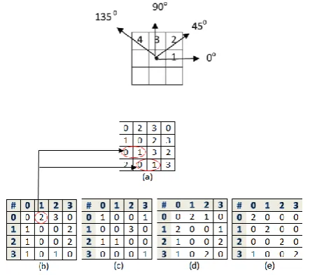
GLCM, which is introduced firstly by Haralick [12], is one of the oldest and prominent statistical textual feature extraction methods [13] applied in many fields [14-17] for texture analysis. GLCM is the matrix that holds the distribution of co-occurring intensity patterns at a given offset over a given image. Second-order statistical (Haralick) features are extracted to analyze the texture of the image, which can subsequently be used for classification tasks [18].

[image:2.595.318.540.423.619.2]

GLCM incorporates the spatial relationships of intensity values with each other as well as their occurrence quantities. Let f is an image whose intensity values vary in the interval [0, L-1]. Each element of GLCM indicates the number of times that the pixel pair (zi, zj) occurred in f with orientation Q. The orientation represented with Q eventually represents a displacement vector d=(dx,dy | dx=dy=dg) where dg is the number of gaps between the pixels of interest. For the situation of adjacency dg=0. Orientation can also be represented with two parameters as the distance d that the intensities zi, zj apart from each other with angle α [19-20]. d can take values between 0 and L-2 theoretically. Orientation of the pixel pattern can be at four different directions as 0°, 45°, 90° and 135° that α can take. That is, each image can have four different GLCMs for each angle (0°, 45°, 90° and 135°) for a specific d. The size of a GLCM depends on the discrete intensity values in the image. If the intensity values of the image vary in the interval [0, L-1] then the size of the GLCM becomes (L-1)×(L-1). An example of configuration of the four GLCM matrixes (GLCM0°, GLCM45°, GLCM90°, GLCM135°) of an image f for d=0 is demonstrated in Figure 2.

Fig 2: GLCM construction based on a (a) test image along four possible directions (b) 0° (c) 45° (d) 90° and (e) 135°

with a distance d =0.

2.3 Haralick Features

Haralick [21] proposed 14 features that can be extracted from the abovementioned GLCMα° matrices. Haralick claimed that

[image:2.595.61.271.542.762.2]

(3)

I

i

I



₁2



₂2



...



_n2



.









n k k k

j

i

1 2

)

(

Angular Second Moment

f

1= N gp(i,j)2 j=1 N g i=1

Contrast _f

2= n2 p(i, j)

Ng

j=1 Ng

i=1 Ng−1

n=0 _{i−j =n}

Correlation _f

3=

(i−μx)(i−μy)(p(i,j)

σxσy

Ng

j=1 Ng

i=1

Sum of Squares f

4= N g i−µ 2_p(i,j) j=1 N g i=1 Inverse Difference Moment

f5=

1

1+(i−j)2p(i, j)

Ng

j=1 Ng

i=1

Sum Average _f

6= ipx+y(i)

2Ng

i=2

Sum Variance _f

7= (i − f8)2px+y(i)

2Ng

i=2

Sum Entropy _f

8= − px+y(i) log px+y(i)

2Ng

i=2

Entropy _f₉_{= − p(i, j) log p(i, j)}

j

i

Difference Variance

f10= variance of px−y

Difference

Entropy f11= − px−y(i) log px−y(i)

Ng−1

i=2

Information Measures of Correlation

f12=

HXY − HXY1 max HX, HY

f13= (1 − exp⁡[−2.0 HXY2

− HXY ])1 2

HXY = − p(i, j) log p(i, j)i j

Maximal Correlation Coefficient

Q i, j = p i,k p(j,k)

px i py(k)

k

f14

= (Second Largest Eigenvalue of Q)1 2

2.4 Euclidean norm

For i = (i1, i2,..., in) and j = (j1, j2,..., jn) are two points in Euclidean n-space, the Euclidean distance d from i to j, or from j to i is given by the Pythagorean formula:

2 2 2 2 2 1

1

)

(

)

...

(

)

(

)

,

(

)

,

(

i

j

d

i

j

i

j

i

j

i

n

j

n

d













(2)

The position of a point in an Euclidean n-space is an Euclidean vector. Euclidean norm, Euclidean length, or magnitude of a vector measures the length of the vector:

(3)

where the last equation involves the dot product.

3. IMPLEMENTATION RESULTS AND

DISCUSSIONS

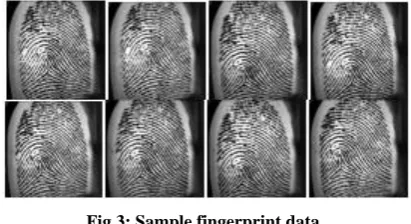
The performance analysis is tested on the IIIT-D SLF fingerprint database [22]. An example of a fingerprint image for an individual is shown in Figure 3.

[image:3.595.49.288.69.493.2]

The utilized database consists of 256x256 RGB coloured images. All RGB images are converted to grey scale format to be compatible with the co-occurrence matrix in the pre-processing stage.

Fig 3: Sample fingerprint data.

The flowchart of the first analysis operation is shown in Figure 4. As shown in the corresponding flowchart, DWT of the images is performed for feature extraction, which is subsequently followed by Euclidean Distance-based classification.

Fig 4: Flowchart of the first analysis.

Figure 5 demonstrates the classification performance for diverse number of training images without applying GLCM. As clarified in this figure, the highest classification accuracy is achieved for 5 training image data.

Fig 5: Classification performance with DWT feature extraction without GLCM.

[image:3.595.326.532.186.298.2] [image:3.595.331.518.475.619.2]

(4)

[image:4.595.54.283.72.167.2]

Fig 6: Flowchart of the second analysis.

[image:4.595.332.520.112.259.2]

In Figure 7, the classification performance of the GLCM feature extraction without DWT is shown. As shown in this figure the highest accuracy is acquired for 7 training image data.

Fig 7: Classification performance with GLCM feature extraction without DWT.

[image:4.595.72.259.238.384.2]

The flowchart of the third analysis method is shown in Figure 8. As shown in this figure GLCM-DWT are used in combination for feature extraction.

Fig 8: Algorithm for GLCM feature extraction with DWT.

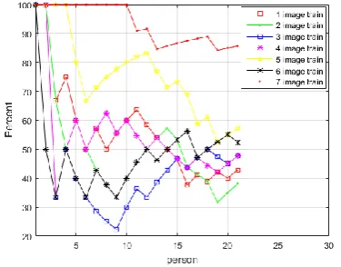
In Figure 9, results for one-level DWT with 8 Haralick features are illustrated. As shown in this figure, the highest accuracy is obtained with 7 training image data.

Fig 9: Classification performance for one-level DWT with 8 Haralick features.

In Figure 10, results for one-level DWT with 6 Haralick features of GLCM are illustrated. As shown in this figure, the highest accuracy is again obtained with 7 training image data.

Fig 10: Classification performance for one-level DWT with 6 Haralick features.

[image:4.595.331.517.331.477.2]

In Figure 11, results for one-level DWT with 4 Haralick features are illustrated. Obviously, again the highest accuracy is achieved with 7 training image data.

[image:4.595.54.280.456.535.2]

In Figure 12, results for one-level DWT with 2 Haralick features are illustrated. As shown in this figure, the highest accuracy is again obtained with 7 training image data.

[image:4.595.334.519.550.697.2] [image:4.595.70.255.591.734.2]

(5)

[image:5.595.70.256.80.228.2]

Fig 13: Classification performance for two-level DWT with 8 Haralick features.

In Figure 14, results for two-level DWT with 6 Haralick features of GLCM are illustrated. As shown in this figure, the highest accuracy is again obtained with 4 training image data.

Fig 14: Classification performance for two-level DWT with 6 Haralick features.

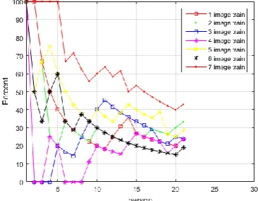
[image:5.595.334.519.134.280.2]

In Figure 15, results for three-level DWT with 8 Haralick features of GLCM are illustrated. As shown in this figure, the highest accuracy is again obtained with 7 training image data.

Fig 15: Classification performance for three-level DWT with 8 Haralick features.

[image:5.595.70.255.305.453.2]

In Figure 16, results for three-level wavelet transform with 6 Haralick are depicted.

Fig 16: Classification performance for three-level DWT with 6 Haralick features.

In Figure 17, results for 14 features with GLCM without DWT are illustrated. As shown in this figure the highest accuracy is obtained for 7 training image data.

Fig 17: Classification performance for 14 features of GLCM without DWT.

4. CONCLUSION

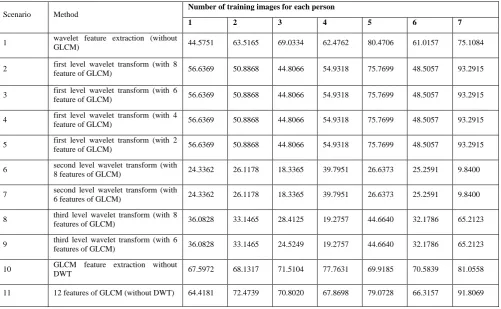
[image:5.595.333.518.354.500.2] [image:5.595.71.254.534.676.2]

(6)

[image:6.595.49.551.87.396.2]

Table 1. Classification Performances

Scenario Method

Number of training images for each person

1 2 3 4 5 6 7

1 wavelet feature extraction (without

GLCM) 44.5751 63.5165 69.0334 62.4762 80.4706 61.0157 75.1084

2 first level wavelet transform (with 8

feature of GLCM) 56.6369 50.8868 44.8066 54.9318 75.7699 48.5057 93.2915

6 second level wavelet transform (with

8 features of GLCM) 24.3362 26.1178 18.3365 39.7951 26.6373 25.2591 9.8400

7 second level wavelet transform (with

6 features of GLCM) 24.3362 26.1178 18.3365 39.7951 26.6373 25.2591 9.8400

8 third level wavelet transform (with 8

features of GLCM) 36.0828 33.1465 28.4125 19.2757 44.6640 32.1786 65.2123

9 third level wavelet transform (with 6 _{features of GLCM)} 36.0828 33.1465 24.5249 19.2757 44.6640 32.1786 65.2123

10 GLCM feature extraction without

DWT 67.5972 68.1317 71.5104 77.7631 69.9185 70.5839 81.0558

11 12 features of GLCM (without DWT) 64.4181 72.4739 70.8020 67.8698 79.0728 66.3157 91.8069

5. ACKNOWLEDGMENTS

Our thanks to the experts who have contributed towards development of the template.

6. REFERENCES

[1] Bowman, M., Debray, S. K., and Peterson, L. L. 1993. Reasoning about naming systems. .

[2] Ding, W. and Marchionini, G. 1997 A Study on Video Browsing Strategies. Technical Report. University of Maryland at College Park.

[3] Fröhlich, B. and Plate, J. 2000. The cubic mouse: a new device for three-dimensional input. In Proceedings of the SIGCHI Conference on Human Factors in Computing Systems

[4] Tavel, P. 2007 Modeling and Simulation Design. AK Peters Ltd.

[5] Sannella, M. J. 1994 Constraint Satisfaction and Debugging for Interactive User Interfaces. Doctoral Thesis. UMI Order Number: UMI Order No. GAX95-09398., University of Washington.

[6] Forman, G. 2003. An extensive empirical study of feature selection metrics for text classification. J. Mach. Learn. Res. 3 (Mar. 2003), 1289-1305.

[7] Brown, L. D., Hua, H., and Gao, C. 2003. A widget framework for augmented interaction in SCAPE. [8] Y.T. Yu, M.F. Lau, "A comparison of MC/DC,

MUMCUT and several other coverage criteria for logical decisions", Journal of Systems and Software, 2005, in press.