The Effect of Time Delay on the Stability of a
Diffusive Eco–epidemiological System
Kejun Zhuang
Abstract—The disease has a vital effect on the dynamical
behaviors of predator-prey system in ecology. When disease spreads in the prey population, the infected preys are more likely to be captured by predators. On the other hand, spatial diffusion and gestation delay are ubiquitous in the nature and can generate rich spatiotemporal dynamical behaviors. In this study, a delayed and diffusive predator-prey system with disease in the prey is proposed. First, the existence, uniqueness, positivity and boundedness of solutions are established. Second, the stability condition of constant predator-free equilibrium solution is derived. Third, the stability of constant coexistence equilibrium solution and the existence of Hopf bifurcation are investigated by regarding time delay as the bifurcation parameter. Finally, some numerical simulations and conclusions are given to illustrate the theoretical results.
Index Terms—eco-epidemiological system, time delay, Hopf
bifurcation, periodic solution.
I. INTRODUCTION
T
HE predator-prey system is the basic model in pop-ulation dynamics, so the interactions between predator and prey in natural ecosystem have drawn extensive attention from scholars in different kinds of fields. As most species are prone to various diseases, abundant improved predator-prey models with disease in the predator-prey or predator have been proposed in the recent past, see [1], [2], [3], [4], [5], [6], [7], [8], [9]. These studies show that the disease in prey or predator species may greatly influence the permanence and stability of the ecosystem, such as the stabilization of predator-prey oscillations, the occurrences of periodic and chaotic oscillations, and so on.Based on the assumption that the plankton species is only a portion of the food for the fish population in lake ecosystem, the overall fish density depends on the productivity of the lake and does not relate directly with plankton density, Bhat-tacharyya and Mukhopadhyay [10] established the following epidemiological model with SIS disease in the population:
( dS
dt =rS 1− S+I
K
−βIpSq−dS+γI, dI
dt =βI
pSq−dI−γI− P I2
I2+
h2,
(1)
where S(t) and I(t) are the densities of susceptible prey and infected prey, respectively. It is assumed that only the susceptible prey is capable of reproducing and its birth rate isr. Infected prey is removed by death or by predation. The disease transmission follows simple mass action law with infected incidence rateβ;pandqare the fractions of infected
Manuscript received February 1, 2018; revised June 16, 2018. K. Zhuang is with the School of Statistics and Applied Mathematics, Anhui University of Finance and Economics, Bengbu, Anhui, 233030 China, e-mail: [email protected]. This work is supported by the youth project of the humanities and Social Sciences in the Ministry of Education (17YJC630175), Anhui Province philosophy and social science planning project(AHSKQ2017D01) and the NSF of Education Bureau of Anhui Province (KJ2017A432).
and susceptible prey population, respectively (0< p, q <1). The prey population has the same natural death ratedand the infected ones suffer additional loss due to recovery at a rateγ and subsequently join the susceptible class. The infected pop-ulation also suffers loss of biomass due to predator pressure at a rate P. The nonnegative initial conditions are imposed and all the coefficients are positive constants. For system (1), the local and global stabilities of various steady states and existence of Hopf bifurcation behavior were investigated by theoretical analyses and numerical simulations.
However, it is more legitimate to consider the impact of predator if the abundance of large piscivorous fish is increas-ing in a lake [11]. Through takincreas-ing account of the density of fish population as a dynamic variable which will significantly influence the dynamics of the system, Chakraborty et al. in [12] considered the extended model as follows:
dS
dt =rS 1− S+I
K
−βIpSq−dS+γI, dI
dt =βI
pSq−dI−γI− mP I2 I2+
h2,
dP dt =
αP I2
I2+h2 −µP −σP 2,
(2)
whereP(t)denotes the density of predator population,µand σP2 are the natural death rate and the density-dependent mortality rate of predator, respectively. It is a well known fact that the infected prey is more vulnerable and it is assumed that the predator only consumes the infected one. The coefficient m is the maximal per capita consumption rate of infected prey, h represents the amount of infected prey at which predation rate is maximal andαrepresents the conversion efficiency of consumed prey into new predator. By regarding the infected incidence rateβ as the bifurcation parameter, Chakraborty et al. [12] examined the existence of Hopf bifurcation around the coexisting equilibrium and discussed the uniform strong persistence of the system.
In fact, spatial diffusion process is ubiquitous. The major-ity of populations do not stay in a fixed place and will move from one place to another driven by the outside influences. Spatial diffusion factor can also generate rich dynamics. For instance, stationary pattern, Hopf bifurcation, Turing instability and pattern formation have been recently studied in [13], [14], [15], [16]. On the other hand, time-delay factor cannot be ignored, because the density of predator is closely related to the state at some time before due to the food supply, competition, sexual maturity, and so on. By introducing time delay, ecologists are able to successfully explain regular population cycles.
Nevertheless, there have been comparatively rare results on such eco-epidemic models taking account of both spatial diffusion and time delay. For instance, Mukhopadhyay and Bhattacharyya [17] considered a delay-diffusion predator-prey model with disease in the predator-prey and Holling type-II functional response. They only discussed the linear stabil-ity of boundary equilibrium and the dissipativeness of the
IAENG International Journal of Applied Mathematics, 48:4, IJAM_48_4_05
system. Crauste et al. [18] introduced a delay reaction-diffusion model of the interaction between susceptible fish and bacterium without predator, and analyzed the stability of uniform steady states and existence of Hopf bifurcation. Zhang et al. [19] established a reaction-diffusion model with disease in the prey and ratio-dependent Michaelis-Menten functional response. They considered the temporal-spatial delay and investigated the dynamic properties. Therefore, it is necessary to further study the joint effects of diffusion and delay on the eco-epidemiological systems.
Motivated by the work of [10], [12], [17], [19], in the present paper, we mainly consider the reaction-diffusion predator-prey with disease in the prey and gestation time delay as follows:
∂S(x,t)
∂t = ∆S(x, t) +rS(x, t)
1−S(x,t)+KI(x,t)
−(βI(x, t) +d)S(x, t) +γI(x, t), x∈Ω, t >0,
∂I(x,t)
∂t = ∆I(x, t) +I(x, t)(βS(x, t)−d−γ) −mPI2((x,tx,t))+I2(hx,t2 ), x∈Ω, t >0,
∂P(x,t)
∂t = ∆P(x, t) +
αP(x,t−τ)I2 (x,t−τ)
I2(x,t−τ)+h2
−µP(x, t−τ)−σP2(x, t−τ), x∈Ω, t >0,
∂S(x,t)
∂n =
∂I(x,t)
∂n =
∂P(x,t)
∂n = 0, x∈∂Ω, t >0,
S(x, t) =S1(x, t)≥0, x∈Ω, t∈[−τ,0], I(x, t) =I1(x, t)≥0, x∈Ω, t∈[−τ,0], P(x, t) =P1(x, t)≥0, x∈Ω, t∈[−τ,0],
(3) whereS(x, t),I(x, t)andP(x, t), respectively, represent the densities of susceptible prey, infected prey and predator at the locationx∈Ωand timet;τ >0is the time required for the gestation of the predator. The region Ω⊂RN(N ≤3)
denotes a bounded domain with smooth boundary ∂Ω; ∆ is the Laplace operator;∂/∂nindicates the outward normal derivative on ∂Ω. The system is subject to homogeneous Neumann boundary conditions, which means that the eco-epidemiological system is self contained and the populations cannot cross the boundary. Unlike the infection incidence function in systems (1) and (2), here, we adopt the classic bilinear functionβSI for simplicity.
The main purpose of this paper is to provide a new perspective for both ecologists and mathematicians. More concretely, we shall focus on the asymptotic stability of the predator-free and coexisting steady states, and the existence of Hopf bifurcation around the coexisting steady state in-duced by time delay. The rest of the paper is organized as follows. In Section 2, we investigate the fundamental properties of solutions for system (3). In Section 3, we carry out the linear stability of two uniform steady states and the existence of Hopf bifurcation by analyzing the corresponding characteristic equations. In Section 4, we conduct some numerical simulations in support of the analytical findings. Finally, we draw some conclusions in the Section 5.
II. FUNDAMENTAL PROPERTIES OF SOLUTIONS In this section, we shall establish the well-posedness of solutions for system (3), including the existence, uniqueness, positivity and boundedness of the solutions.
First, we denote the Banach space of continuous functions from[−τ,0]intoX with the usual supremum norm byC= C([τ,0], X). In our case, X is the Banach spaceC(Ω,R3) and C(E, F) represents the space of continuous functions
from topological spaceEinto spaceF. For convenience, we identify an element ϕ∈C as a function from Ω×[−τ,0] intoR3 defined byϕ(x, s) =ϕ(s)(x).
For any continuous functionw(.) : [−τ, b)→X forb >0, we define wt ∈ C bywt(s) = w(t+s), s ∈[−τ,0]. It is
easy to find thatt→wtis a continuous function from[0, b)
toC.
Proposition 1 For any nonnegative initial conditions of system (3), there exists a unique solution and this solution remains nonnegative and bounded for anyt≥0.
Proof of Proposition 1: For anyϕ= (ϕ1, ϕ2, ϕ3)T ∈C andx∈Ω, we defineF = (F1, F2, F3) :C→X by
F1(ϕ)(x) =rS(x,0)
1−S(x,0) +KI(x,0)
−(βI(x,0) +d)S(x,0) +γI(x,0),
F2(ϕ)(x) =I(x,0)(βS(x,0)−d−γ)−
mP(x,0)I2(x,0) I2(x,0) +h2 ,
F3(ϕ)(x) =αP(x,−τ)I
2(x,−τ)
I2(x,−τ) +h2 −µP(x,−τ)
−σP2(x,−τ).
Then, system (3) can be rewritten as the abstract functional differential equation:
w′(t) =Aw+F(w
t), t >0,
w(0) =φ∈X, (4)
where
w= (S, I, P)T,
φ= (S1, I1, P1)T, Aw= (∆S,∆I,∆P)T.
It is clear thatF is locally Lipschitz inX. According to the results in [20], [21], [22], [23], [24], we can conclude that system (4) admits a unique local solution on[0, Tmax),
where Tmax is the maximal existence time for solution of
system (4).
Besides, we can also obtain thatS(x, t)≥0,I(x, t)≥0 andP(x, t)≥0becauseO= (0,0,0)is a lower solution of system (3).
Next, we verify the boundedness of solutions. In fact, we only need to prove that any solution is uniformly bounded. It is easy to see thatM= (M1, M2, M3)is a upper solution of system (3), where
M1= max
K, sup −τ≤t≤0k
S1(·, s)kC(Ω,R)
,
M2= max
K, sup −τ≤t≤0k
I1(·, s)kC(Ω,R)
,
M3= max
α
σh2, sup −τ≤t≤0k
P1(·, s)kC(Ω,R)
.
Based on the comparison principle, we have
0≤S(x, t)≤M1,0≤I(x, t)≤M2,0≤P(x, t)≤M3
for x ∈ Ω and t ∈ [0, Tmax). Then the solutions of (3)
are bounded on Ω×[0, Tmax). From the stand theory for
semilinear parabolic systems in [25], we deduce thatTmax=
+∞. The proof is complete.
IAENG International Journal of Applied Mathematics, 48:4, IJAM_48_4_05
III. STABILITY OF UNIFORM STEADY STATES As we know, spatial diffusion and time delay do not change the number and location of the uniform steady states. With the similar method in [12], we can obtain the predator-free equilibriumE0= (S0, I0,0)and the coexisting equilibriumE∗= (S∗, I∗, P∗), where
S0= d+γ β ,
I0=
(d+γ)(Kβr−Kβd−rd−rγ) β(Kβd+rd+rγ) ,
S∗=
√
b2−4ac−b 2a ,
P∗= 1 σ
αI∗2 I∗2+h2 −µ
,
a=r,
b=rI∗+βKI∗+dK
−Kr, c=−γKI∗,
andI∗ is the positive root of the following equation
r
1−I
∗ K −
d+γ+ mαI ∗3 σ(I∗2+h2)2 −
mµI σ(I∗2+h2)
−d+γI∗
d+γ+ mαI ∗3 σ(I∗2+h2)2 −
mµI σ(I∗2+h2)
−1
= 0.
Next, we will investigate the asymptotic stability of the two uniform steady states.
We first introduce some useful concepts from [24]. Let0 = µ0< µ1< µ2<· · · denote the eigenvalues of the operator
−∆inΩunder homogeneous Neumann boundary conditions and s(µk) be the eigenfunction space corresponding to µk
with dimension numbernk = dim[s(µk)]inC1(Ω).
(i) Xk:={Pnk
j=1cjϕkj :cj∈R}, where{ϕkj}nj=1k are an orthogonal basis ofs(µk).
(ii) X:={(S, I, P)∈ C1(Ω)×C1(Ω)×C1(Ω) : ∂S ∂n =
∂I ∂n =
∂P
∂n = 0 on ∂Ω}, so thatX=
L∞
k=0Xk.
A. Stability of predator-free equilibrium
Theorem 1 If Kβr > Kβd+rd+rγ, then for anyτ≥
0, the predator-free equilibriumE0 is asymptotically stable whenαI2
0 < µ(I02+h2)or unstable whenαI02> µ(I02+h2). Proof of Theorem 1: The linearization of system (3)
at the predator-free equilibrium E0 = (S0, I0,0) can be expressed by
Yt= (E∆ +FY(E0))Y,
whereEis the unit matrix,Y = (S(x, t), I(x, t), P(x, t))T,
and
FY(E0)
=
−γI0
S0 −
rS0
K −
r(d+γ)
Kβ −d 0
βI0 0 −ImI2 0
0+h 2
0 0 αI
2 0
I2 0+h
2e
−λτ−µ
.
Fork ≥0, it is observed that Xk is invariant under the
operator E∆ +FY(E0) and λ is an eigenvalue of E∆ + FY(E0) on Xk if and only if λ is an eigenvalue of the
matrix−µkE+FY(E0). That is
λ+µk−
αI2 0 I2
0+h2
e−λτ+µ
h
λ2+2µ
k+γIS00+
rS0
K
λ
+µ2k+µk
γI0 S0
+rS0 K
+r(d+γ)I0
K +dβI0
= 0.
It is apparent that all roots of the quadratic equation
λ2+
2µk+γI0
S0 + rS0
K
λ+µ2k
+µk
γI0 S0
+rS0 K
+r(d+γ)I0
K +dβI0= 0
must have strictly negative real parts. Then we only need to consider the following transcendental equation:
λ+µk−
αI2 0 I2
0+h2
e−λτ+µ= 0. (5)
Whenτ= 0, the root of (5) isλ=−µk+ αI
2 0
I2 0+h
2−µ. We can find thatλ <0 for any k≥0whenαI2
0 < µ(I02+h2), andλ >0 for somek≥0 whenαI2
0 > µ(I02+h2). Whenτ > 0, assume that λ =iω (ω > 0) is a root of (5), and we have
αI2 0 I2
0+h2
(cosωτ−isinωτ) =µk+µ+iω.
Separating the real and imaginary parts leads to
αI2 0 I2 0+h
2cosωτ =µk+µ,
αI02
I2 0+h
2sinωτ =−ω,
and
ω2=
αI2 0 I2
0 +h2
+µk+µ
αI2 0 I2
0 +h2
−µk−µ
. (6)
IfαI02< µ(I02+h2), then equation (6) has no positive root and equation (5) has no purely imaginary root. According to the Corollary 2.4 in [26], as parameter τ varies, the sum of the orders of the roots of (5) in the open right half plane can change only if a root appears on or crosses the imaginary axis. As a consequence, equation (5) has roots only with negative real part if the conditionαI2
0 < µ(I02+h2) holds. It is known that the constant equilibrium solution is asymptotically stable only if all the characteristic values have strictly negative parts. Thus, the proof is complete.
The asymptotic stability of predator-free equilibrium im-plies the extinction of predator. Therefore, from Theorem 1, it can be observed that the predator population may extinct when its death rate µ is large or the conversion efficiency coefficientαis sufficiently small.
B. Existence of Hopf bifurcation around the positive equi-librium
The asymptotic stability of positive equilibrium implies the coexistence of both predator and prey species, which
IAENG International Journal of Applied Mathematics, 48:4, IJAM_48_4_05
would be helpful for the population conservation and the sustainable development of ecosystem. Consequently, we are more interested in the effect of time delay on the stability of the coexisting equilibrium E∗. Here, we concentrate on the stability of positive equilibrium and the existence of Hopf bifurcation by regarding time delayτ as the bifurcation parameter.
Linearizing system (3) at the positive equilibriumE∗, we can obtain the characteristic equation
λ+µk+a11 a12 0
a21 λ+µk+a22 a23
0 a32e−λτ λ+µk+a33e−λτ+b33
= 0,
(7) where
a11= γI∗
S∗ + rS∗
K ,
a12= r KS
∗+βS∗
−γ,
a21=−βI∗,
a22= mP ∗I∗ I∗2+h2−
2mp∗I∗3 (I∗2+h2)2,
a23=m(µ+σ)
α ,
a32= 2αh 2P∗I∗2 (I∗2+h2)2,
a33=− αI ∗2 I∗2+h2, b33=µ−2σP∗.
Then the characteristic equation (7) can be reduced to
λ3+Akλ2+Bkλ+Ck+e−λτ(Dkλ2+Fkλ+Gk) = 0, (8)
where
Ak = 3µk+a11+a22+b33,
Bk = 3µ2k+ 2(a11+a22+b33)µk+a11a22
+a22b33+a11b33−a12a21,
Ck=µ3k+ (a11+a22+b33)µ2k+ (a11a22+a11b33
+a22b33−a12a21)µk+a11a22b33−a12a21b33,
Dk=a33,
Fk= 2a33µk+a11a33+a22a33−a23a32,
Gk=a33µ2k+ (a11a33+a22a33−a23a32)µk
+a11a22a33−a11a23a32−a12a21.
The expressions of the coefficients in equation (8) are too complex, so we can only derive the general conditions for stability of the positive equilibriumE∗. The detailed numer-ical calculations will be left in the next section. Then, we discuss the distribution of characteristic values in equation (8).
Forτ = 0, the characteristic equation (8) can be rewritten as
λ3+ (Ak+Dk)λ2+ (Bk+Fk)λ+ (Ck+Gk) = 0. (9)
By Routh-Hurwitz criterion, all roots of the cubic equation (9) have strictly negative real parts if and only if the following conditions hold:
(H1) Ak+Dk>0;
(H2) Bk+Fk>0;
(H3) Ck+Gk >0;
(H4) (Ak+Dk)(Bk+Fk)−(Ck+Gk)>0.
Given this, the positive coexisting equilibriumE∗ is locally asymptotically stable without time delay.
On the other hand, we discuss the effect of time delayτon the stability of the positive equilibrium. Assume thatλ=iω (ω >0)is a root of (8). Substituting it into the equation can yield
−iω3−A
kω2+iBkω+Ck
+(−Dkω2+iFkω+Gk)(cosωτ−isinωτ) = 0.
(10)
Segregating the real and imaginary parts of equation (10), we have
(Dkω2−Gk) sinωτ+Fkωcosωτ =ω3−Bkω,
Fkωsinωτ −(Dkω2−Gk) cosωτ =Akω2−Ck.
(11) Taking square on both sides of the equations of (11) and summing them up, we can obtain
ω6+ (A2
k−2Bk−D2k)ω4+Qkω2+Ck2−G2k = 0, (12)
whereQk =Bk2−2AkCk+ 2DkGk−Fk2.
Letz=ω2, then equation (12) can be transformed into a cubic equation ofzin the form of
Λ(z) =z3+(A2k−2Bk−D2k)z2+Qkz+Ck2−G2k = 0. (13)
We make the following hypothesis: (H5) Ck−Gk <0.
Assume that(H3)and(H5)hold. It is easy to show that C2
k−G
2
k <0. Hence, equation (13) has at least one positive
root due to the Descartes’ rule of singes [27]. Without loss of generality, we assume that equation (13) has three positive roots and denote any one by z∗. Then equation (12) has positive root ω∗ = z∗2, from which we can deduce that the characteristic equation (8) may have a pair of purely imaginary rootsλ=±iω∗ under certain condition.
Solving the equations of (11), we get
cosωτ = (Fk−AkDk)ω 4
+(AkGk+CkDk−BkFk)ω 2
−CkGk
F2 kω
2
+(Dkω2−Gk)2 , sinωτ = Dkω
5
+(AkFk−BkDk−Gk)ω 3
+(BkGk−CkFk)ω
F2 kω
2+(
Dkω2−Gk)2 . Therefore, if we denote
τ∗
j =
1 ω∗
arccos(Fk−AkDk)ω 4+S
kω2−CkGk
F2
kω2+ (Dkω2−Gk)2
,
whereSk =AkGk+CkDk−BkFkandj= 0,1,2,· · ·, then ±iω∗is a pair of purely imaginary roots of (8) atτ =τ∗
j.
IAENG International Journal of Applied Mathematics, 48:4, IJAM_48_4_05
To guarantee the occurrence of Hopf bifurcation, we still need to verify the transversal condition. Taking the derivatives of (8) with respect toτ results in
dλ dτ
−1
= 3λ 2+ 2A
kλ+Bk+e−λτ(2Dkλ+Fk)
λe−λτ(D
kλ2+Fkλ+Gk) −
τ λ.
(14)
Substituting λ=iω∗andτ =τ∗
j into (14), we have
d(Reλ(τ)) dτ
−1
λ=iω∗,τ=τ∗ j
= HK−LT ω∗2(J2+K2),
where
H =−3ω∗2+B
k,
J = 2Akω∗,
K=Gk−Dkω∗2,
L=Fkω∗,
M =Hsinω∗τ∗
j +Jcosω∗τj∗+ 2Dkω∗,
T =Hcosω∗τ∗
j −Jsinω∗τj∗+Fk.
Then we can obtain the transversal condition
d(Reλ(τ)) dτ
−1
λ=iω∗,τ=τ∗ j
>0
when the following inequality (H6) HK−LT >0
is satisfied.
Again based on the significant results in [26], we can find that if the assumptions (H1)−(H6) are satisfied, then all roots of characteristic equation (8) have negative real parts forτ ∈[0, τ∗
0). Moreover, a pair of purely imaginary roots exist for τ=τ∗
0 and a pair of roots with positive real parts will appear for τ > τ∗
0. By applying the Hopf bifurcation theorem in [24], the conclusions about the stability of pos-itive equilibrium and existence of the Hopf bifurcation can be drawn as follows.
Theorem 2 If the assumptions (H1) − (H6) are all satisfied, then the following statements are true.
(i) The positive equilibrium E∗ is locally asymptotically stable whenτ∈[0, τ∗
0).
(ii) The positive equilibrium E∗ is unstable when τ > τ∗
0. The Hopf bifurcation occurs at τ =τ0∗. That is, system (3) has a series of periodic solutions aroundE∗ whenτ is slightly larger thanτ∗
0.
IV. NUMERICALSIMULATIONS
In this section, we shall give some numerical examples to describe the previous theoretical results with the help of Mathematica and MATLAB. Here, we consider the system in one dimensional space Ω = (0, π)for simplicity.
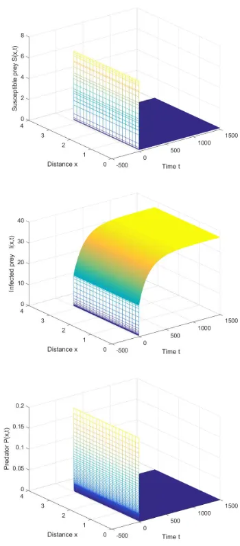
First, we choose
r= 1.5, K = 100, d= 0.003, γ= 0.05, α= 0.09,
µ= 0.5, σ= 0.1, h= 15, β= 0.45, m= 1.5, τ = 2.5.
[image:5.595.339.514.58.456.2]Then the predator-free equilibrium is E0 = (0.1178,36.9452,0), and the conditions in Theorem 1
Fig. 1. The predator-free equilibrium is stable whenτ= 2.5.
are satisfied. It is to be noted that the boundary equilibrium E0 is asymptotically stable (see Figure 1).
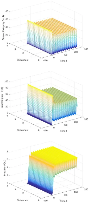
Second, we rechoose
r= 1.5, K = 100, d= 0.03, γ= 0.05, α= 0.9,
µ= 0.001, σ= 0.1, h= 15, β= 0.45, m= 1.5.
Then the coexisting equilibrium is E∗ = (9.8745,24.7625,6.2011). We can also derive the first Hopf bifurcation critical value τ∗
0 = 1.61 for k = 0. When time delay is smaller than the critical value, the positive equilibrium is asymptotically stable (see Figure 2). Otherwise, when time delay is slightly larger than the critical value, the positive equilibrium becomes unstable and periodic solution will bifurcate fromE∗ (see Figure 3).
V. CONCLUSIONS
In this paper, we have considered a delay-diffusion predator-prey system with disease in the prey. The model, which incorporates the spatial diffusion and time delay effects, is much more generalized than those in [10], [12]. As pointed in [12], the consideration of a disease in the prey or predator population makes the system extremely complex.
IAENG International Journal of Applied Mathematics, 48:4, IJAM_48_4_05
Fig. 2. The positive equilibrium is stable whenτ= 0.3< τ∗ 0.
Despite all this, the dynamical behaviors in such systems still have a guidance function to the ecological diversity.
It is observed from our results that the uniform predator-free steady state is asymptotically stable under certain con-dition, but the stability has nothing to do with the gestation delay. However, this stability is harmful, as the predator population will be ultimately extinct over time. To avoid this phenomenon, some measures may be taken to reduce the mortality of predator population or increase the food sources. It can also be observed that the gestation delay has crucial impact on the asymptotic stability of the uniform coexisting steady state. The stability of positive equilibrium is not affected by time delay when it is sufficiently small. However, the stability changes when the gestation delay is larger than some critical value and spatially periodic solution will arise. According to these facts, we can know that both time delay and spatial diffusion can generate periodic pattern and play an important role in spatiotemporal dynamics. Therefore, in order to maintain the stability of the ecosystem, it is better to shorten the gestation delay of predator population.
Of course, the methods and results in this paper can be applied to other reaction-diffusion systems. We hope that our work could be instructive to both theoretical and applied
Fig. 3. The positive equilibrium is unstable and periodic solution appears whenτ= 2.5> τ∗
0.
ecologists.
REFERENCES
[1] J. Chattopadhyay and O. Arino, “A predator-prey model with disease in the prey,” Nonlinear Analysis, vol. 36, no. 6, pp. 747-766, 1999. [2] Y. N. Xiao and L. S. Chen, “Modeling and analysis of a predator-prey
model with disease in the prey,” Mathematical Biosciences, vol. 171, no. 1, pp. 59-82, 2001.
[3] M. Haque and E. Venturino, “The role of transmissible diseases in the Holling-Tanner predator-prey model,” Theoretical Population Biology, vol. 70, no. 3, pp. 273-288, 2006.
[4] F. M. Hilker and K. Schmitz, “Disease-induced stabilization of predator-prey oscillations,” Journal of Theoretical Biology, vol. 255, no. 3, pp. 299-306, 2008.
[5] G. P. Hu and X. L. Li, “Stability and Hopf bifurcation for a delayed predator-prey model with disease in the prey,” Chaos, Solitons and
Fractals, vol. 45, no. 3, pp. 229-237, 2012.
[6] W. J. Du, S. Qin, J. G. Zhang and J. N. Yu, “Dynamical behavior and bifurcation analysis of SEIR epidemic model and its discretization,”
IAENG International Journal of Applied Mathematics, vol. 47, no. 1,
pp. 1-8, 2017.
[7] K. Das, “Disease-induced chaotic oscillations and its possible control in a predator-prey system with disease in predator,” Differential
Equations & Dynamical Systems, vol. 24, no. 2, pp. 215-230, 2016.
[8] H. Singh, J. Dhar and H. S. Bhatti, “Dynamics of a prey-generalized predator system with disease in prey and gestation delay for predator,”
Modeling Earth Systems & Environment, vol. 2, no. 2, pp. 1-9, 2016.
IAENG International Journal of Applied Mathematics, 48:4, IJAM_48_4_05
[image:6.595.86.257.62.459.2][9] S. Olaniyi, M. A. Lawal and O. S. Obabiyi, “Stability and sensitiv-ity analysis of a deterministic epidemiological model with pseudo-recovery,” IAENG International Journal of Applied Mathematics, vol. 46, no. 2, pp. 160-167, 2016.
[10] R. Bhattacharyya and B. Mukhopadhyay, “On an epidemiological model with nonlinear infection incidence: Local and global perspec-tive,” Applied Mathematical Modelling, vol. 35, no. 7, pp. 3166-3174, 2011.
[11] S. R. Carpenter, J. F. Kitchell and J. R. Hodgson, “Cascading trophic interactions and lake productivity,” Bioscience, vol. 35, no. 10, pp. 634-639, 1985.
[12] K. Chakraborty, K. Das, S. Haldar and T. K. Kar, “A mathematical study of an eco–epidemiological system on disease persistence and extinction perspective,” Applied Mathematics and Computation, vol. 254, pp. 99-112, 2015.
[13] J. J. Li and W. J. Gao, “Analysis of a prey-predator model with disease in prey,” Applied Mathematics and Computation, vol. 217, no. 8, pp. 4024-4035, 2010.
[14] X. S. Tang and Y. L. Song, “Stability, Hopf bifurcations and spatial pat-terns in a delayed diffusive predator-prey model with herd behaviour,”
Applied Mathematics and Computation, vol. 254, pp. 375-391, 2015.
[15] H. Y. Zhao, X. X. Huang and X. B. Zhang, “Turing instability and pattern formation of neural networks with reaction-diffusion terms,”
Nonlinear Dynamics, vol. 76, no. 1, pp. 115-124, 2014.
[16] T. Wang, “Pattern dynamics of an epidemic model with nonlienar incidence rate,” Nonlinear Dynamics, vol. 77, no. 1-2, pp. 31-40, 2014. [17] B. Mukhopadhyay and R. Bhattacharyya, “Dynamics of a delay-diffusion prey-predator model with disease in the prey,” Journal of
Applied Mathematics and Computing, vol. 17, no. 1-2, pp. 361-377,
2005.
[18] F. Crauste, M. L. Hbid and A. Kacha, “A delay reaction-diffusion mod-el of the dynamics of botulinum in fish,” Mathematical Biosciences, vol. 216, no. 1, pp. 17-29, 2008.
[19] X. L. Zhang, Y. H. Huang and P. X. Weng, “Stability and bifurcation of a predator-prey model with disease in the prey and temporal-spatial nonlocal effect,” Applied Mathematics and Computation, vol. 290, pp. 467-486, 2016.
[20] C. C. Travis and G. F. Webb, “Existence and stability for partial functional differential equations,” Transactions of the American
Math-ematical Society, vol. 200, no. 7, pp. 395-418, 1974.
[21] W. E. Fitzgibbon, “Semilinear functional differential equations in Banach space,” Journal of Differential Equations, vol. 29, no. 1, pp. 1-14, 1978.
[22] R. H. Martin and H. L. Smith, “Abstract functional differential equa-tions and reaction-diffusion systems,” Transacequa-tions of the American
Mathematical Society, vol. 321, no. 1, pp. 1-44, 1990.
[23] R. H. Martin and H. L. Smith, “Reaction-diffusion systems with time delays: monotonicity, invariance, comparison and convergence,” J.
Reine Anges. Math., vol. 413, pp. 1-35, 1991.
[24] J. H. Wu, Theory and Applications of Partial Functional Differential
Equations. New-York: Springer-Verlag, 1996.
[25] D. Henry, Geometric theory of semilinear parabolic equations. New-York: Springer-Verlag, 1993.
[26] S. G. Ruan J. J. Wei, “On the zeros of transcendental functions with applications to stability of delay differential equations with two delays,” Dynamics of Continuous, Discrete and Impulsive Systems
Series A: Mathematical Analysis, vol. 10, no. 6, pp. 863-874, 2003.
[27] R. Descartes, The Philosophical Writings of Descartes. Cambridge: Cambridge University Press, 1985.
[28] S. N. Wu, J. P. Shi and B. Y. Wu, “Global existence of solutions and uniform persistence of a diffusive predator-prey model with prey-taxis,” Journal of Differential Equations, vol. 260, no. 7, pp. 5847-5874, 2016.
[29] J. M. Lee, T. Hillen and M. A. Lewis, “Pattern formation in prey-taxis system,” Journal of Biological Dynamics, vol. 3, no. 6, pp. 551-573, 2009.