Munich Personal RePEc Archive
Forecasting Inflation using Functional
Time Series Analysis
Zafar, Raja Fawad and Qayyum, Abdul and Ghouri, Saghir
Pervaiz
Lecturer Shaheed Bynazir Bhutto University, Shaheed Bynanirabad,
Nwabshah, Sindh, Pakistan, Joint Director, Pakistan Institute of
Developmental Economics, Islamabad, Pakistan, Joint Director,
State Bank of Pakistan, Karachi, Pakistan.
20 March 2015
Online at
https://mpra.ub.uni-muenchen.de/72002/
1
Introduction
In every real life phenomenon there is an uncertainty involved. We want to
model this uncertainty for some reasons. One of the reason is forecasting for
the purpose of decision making. If we have some knowledge of the future
then we can make decisions to meet our objectives. Econometrics is used for
modeling this uncertainty, specially in Economics. Making a right decision on
right time is very important to tackle the complex system of Economy. There
are mainly four objectives of the Econometric modeling. First is Describing
a real life phenomenon using some model, secondly Forecasting, thirdly
Ca-sual Analysis and last but not least Policy Analysis, as suggested by Hendry
(1995).
Consumer Price Index (CPI) is a key variable which indicate the overall
price level of basket of goods and services in a country. It has many useful
motives, some are suggested by Khalid and Asghar (2010), as measuring cost
of living, indexation of monetary flows, indexation of wages, indexation of
rents, indexation of social security benefit and inflation. Inflation is one of
the important variable that can influence the whole economy and
individual as well as economy. To maintain a rapid growth in the economy
it is very important to maintain inflation at threshold level. High inflation
with a momentum can be an indication of diluting economy. On the other
hand low inflation may also have negative impact on growth.
Inflation forecasting is equally important for monetary policy as well as fiscal
policy. Private agents, labor market and financial market also react to the
change in inflation. Irrespective of having expectation about inflation, so it is
of grave importance to have accurate forecast to some horizons. Inflation is
very important indicator of a country’s economy. It provides understanding
of the state of economy. Generally economist alleged that high inflation is
caused by the extensive supply of money.It is a main objective of the central
bank to maintain a moderate level of inflation for steady growth of economy.
In Pakistan various factors effect inflation including money supply and fuel
prices. Qayyum (2006) studied some determinants of inflation and found
that in Pakistan it is highly effected by the monetary policy. Recent rise
in inflation has many causes but excessive printing of money by democratic
governments, rise in prices of fuel in international market, rise in price of
elec-tricity, shortage of electricity and rise in production cost are the important
factors influencing the inflation rate. Although there are different studies to
define a threshold level of inflation for which there is a positive impact on
case of developing countries 7-11 percent of inflation is claim to be a level for
which there is a positive impact as noted by Khan and Senhadji (2001). In
case of Pakistan it is found that inflation around 8 percent is best .
Forecasting is one of the main objectives of Econometric modeling. There are
mainly two types of forecasting. Statistical forecasting i.e. based on
histor-ical data (Univariate models also called extrapolation ) and Economic
fore-casting i.e. based on Multivariate models (VAR models and cointegration).
Univariate models are used for short term forecasting where as multivariate
models are renowned for long term forecasting. Both type of models have
their pros and cons. One may argue that univariate models are same like a
guess which may or may not be true (rather its a scientific guess with some
confidence interval). On the other hand multivariate models are more
com-plex and errors like model mispecification can arise. Another factor which
may add accuracy to forecasting is frequency of the data. High frequency
data can be used to have more accurate forecast. High frequency data has
an advantage of accurate forecast which may induce complexity specially to
multivariate models.
In the present study our main objective is to forecast inflation in case of
Pakistan as accurate as possible. Secondary one is comparing forecasting
performance. For this purpose we are using highest frequency data of
the inflation using classic Box-Jenkins methodology and Functional Time
Se-ries Analysis using data of CPI general from 2002-2011 of Pakistan.
2
Literature Review
In forecasting inflation many efforts have been made using different
vari-ables and methodology. Many authors have used univariate models (ARIMA
and ARCH models), famous Philips curve (VAR models) and cointegration.
Many determinants like unemployment, Economic growth and Monetary
variables like money supply have been used for this purpose. If we study
the evaluation of time series methodologies we found that Wiener (1964)
had pioneer work ,which laid the foundation of modern time series analysis
and forecasting. This work was actually done to resolve some problems in
engineering related to frequency domain. He was trying to estimate under
lying signal for set of time series observations corrupted by noise. These
signal extraction models work almost similar to complex econometric models
in forecasting, developed at different time.
In forecasting time series based on purely statistical or models based on
historical data, many types of modification like , linear, non linear,
ARIMA models developed by US Bureau forecast after extracting the cyclical
and seasonal component. Exponential smoothing is another method used to
forecast variable’s future values. Originally it was developed by Holt (1957)
and then Winters (1960) applied this technique to forecast sales. He also
introduced a slope term in the model. The main idea behind exponential
smoothing was to give exponential weights to the observations based their
time of occurrence. The most recent observation has the maximum weight
and rest have exponentially decaying weights with the minimum weight to
the first observation. The advantage of this technique is it minimizes the
inherited noise in the observation which leads to a smooth curve. This curve
made by exponential smoothing is then used to forecast future values. The
main disadvantage of this method is that it lacks the theoretical consideration
due to which it doesn’t allow for prediction interval.Brown and Meyer (1961)
studied the least square estimated of coefficients of exponential smoothing
model.His contribution added the flavor of econometrics in the model Many
other contributions were made till 1970 in existing as well as new techniques.
In the same year Box and Jenkins (1970) came up with a methodology that
address many practical issues for modeling and forecasting time series.
In case of multivariate forecasting techniques first one is a multivariate
ex-tension of ARIMA model i.e. Vector ARIMA models. Vector Autoregressive
(1968). In general The main disadvantage of the VAR model is, that it has
too many extra estimated parameters which are usually insignificant , as a
re-sult out of sample forecasting is poor as noted by Simkins (1995) although in
sample forecasting is good. Performance of VAR models were even worst at
level when variables involved are non stationary. Engle and Granger (1987)
comes up with a solution called cointegration and Error Correction models.
These models have good out sample forecasting on the long horizon. Some
modified and improved versions of the method are also available. Besides
these some non linear models like regime switching models, Artificial Neural
Network models, GARCH models and ARFIMA models are also used for
forecasting purpose.
Comparison of forecast efficiency of different type of models have been
made in many studies. Cooper (1972) and Naylor et al. (1972) concluded
that ARIMA models performance is superior then Wharton Economic model.
Armstrong (1985) in his famous book compared the performance of both type
of models and concluded that time series models are superior then Economic
models. Specifically in univariate vs economic forecasting. Meyler et al.
(1998)found that ARIMA models outperform all other models in
forecast-ing Irish inflation. They also investigated the performance of VAR models
out-perform models like Philip’s curve. Stockton and Glassman (1987) showed
that time series ARIMA models outperform macro models. In a paper by
Lee (2012), predictive performance of the univariate time series and some
economic forecast models were compared. He found that univariate models
are the optimal ones for forecasting inflation.
In the early history of Pakistan till 1990 inflation was not a big issue.
After the adoption of Structural Adjust Program in 90’s the focus shifted
on this side. The main debate started after 2000 about inflation, monetary
variables and policy. Before 2000 we have few studies in this context. After
it many studies have been made specially focused on inflation and monetary.
The main focus of the studies was to determining the possible variable
re-sponsible for change in inflation. These multivariate studies was of two type.
Theoretical (Economic Forecasting)and models just for forecasting inflation
with out any theory based analysis (Statistical Forecasting). Most of the
work done in theory based model was to test monetary theory or checking
possible determinants of inflation.
For example Ahmed [1991] found Gross National product (GNP), growth
rate of imports, growth in ratio of M1 and M2 as important variables in
determining inflation. Dhakala[1993] found M1 , interest rate import prices
variables. Ahmed and Ali [1999] finds interest rate as important one. Khan
[2002] finds Dollar exchange rate, Khalid 2005 suggest imported inflation
and openness important. Malik [2006] founds money supply as more
influ-ential. Aleem [2007] conclude adaptive expectation private sector credit and
imported prices as one of possible causes of inflation. Omer and Farooq
[2008] and Khan et. al [2008] tested and concluded political instability as
most influential on unstable price level. Some of the researchers tested some
theories. Akhter [1990] supported monetarist point of view in determining
inflation. Bayer[1993], Qayyum [2006] and Kemal[2006] found evidence in
favor of Quantity Theory of Money. On the other hand some studies are
also their for multivariate case in forecasting inflation of Pakistan. Different
models have been used for example Ahmed [1999] used 2sls method. Hyder
and Shah used Recursive VAR model. Qayyum [2005] built a p-star model.
Khan [2006] and Kemal [2006] used VECM for the purpose of forecasting.
Gul [2012] using data 1992-2010 finds Philips Curve still good to forecast
in-flation in Pakistan. Tahir et. al [2014] used data from 1991-1 to 2013-11 and
Bayesian VAR modle to forecast inflation of Pakistan. He used three priors
for this purpose. Minnesota, Independent Normal-Wishart and Independent
Minnesota Wishart priors.
In the past fifteen years there are numerous fields in which Functional Data
Demographic forecasting, Human growth, multi-stream web data, Ecology ,
Environment studies and many more see (ullah [2013]). It is mainly consist
of smoothing techniques, data reduction techniques, functional linear models
and forecasting methods. In demography age specific mortality rates,
Hynd-man and Shang (2010), fertility, mortality and HyndHynd-man and Booth (2008),
monthly non-durable goods index Ramsay and Ramsey (2002) and income
distribution.
Particularly in foretasting inflation Chaudhuri et al. applied the functional
data method on forecasting inflation. He used Sector wise disaggregated data
of CPI in two and more levels. He used data of CPI disaggregated at 2nd and
3rd level from January 1997 to February 2008. Authors modeled Each series
of disaggregated data as a functional observation. After smoothing the data
using kernel smoothing methods, Functional Autoregressive model(FAR) was
fitted. Recomposing each level of forecasted data series to get next level
se-ries using some weights and finally getting CPI. Authors fitted many model
to forecast the series after smoothing. FAR(1), fitting FAR after differencing
(DFAR), FAR on 3 month moving average (3m). Authors found
FAR-3m model to be optimal in forecasting inflation.
In case of Pakistan many attempts have been made for forecasting inflation.
Forecasting inflation using time series models were attempted by many
to 2004-6. He fitted many ARIMA models using Box-Jenkins methodology.
Author compared performance of all these univariate models using
perfor-mance evaluation criteria. Haider and Hanif (2009) foretasted inflation using
Artificial neural networks. Iftakhar and Amin (2013) modeled the data
1961-2013 of CPI using ARIMA models foretasted the inflation of Pakistan to be
8.83 in year 2013. They found ARIMA(1,1,1) model the best for forecasting
inflation. Sultana et al. (2013) used monthly data of CPI from 2008-7 to
2013-6. Authors modeled the data using two methods . ARIMA models and
decomposing CPI to its time series components and then recomposing after
projection to forecast inflation. They concluded that the ARIMA models
gives better results.
3
Methodology and Data
In this section we will briefly explain the functional data analysis and its
application to forecasting Functional Time Series Analysis (FTSA). In
3.1
ARMA Models
The autoregressive model is a kind of linear regression in which independent
variables is actually the response variable from the previous period (i.e. lag
of the series). For example for a series yt, the autoregressive of order p (i.e.
AR(p) ) is of the form
yt=φ1yt−1+φ2yt−2, ..., φpyt−p+ǫt (1)
where ǫt is noise in the data series assumed to be identically independently
distributed with 0 mean. The reason to denote AR(p) is that yt is regressed
on its own subsequent previous years values.The moving average is a linear
model of a time series dependent on the past errors. So the MA model of
order q an be expressed as
yt=θ1ǫt−1+θ2ǫt−2 +...+θqǫt−q (2)
3.1.1 Test for Structural Break
We have used in this thesis Bai and Perron (1998) test for structural breaks.
The standard model considered by authors is a multiple linear regression
m+ 1 regimes. The model is given by
Y =Xβ+Zδ+ǫ (3)
where Z is a set of variables whose coefficient vary across regimes and X is
set of variable whose coefficients remain same across the regimes.We have
used here sequential procedure so we will only define it. The steps involved
in the testing are following. First full sample is considered and consistency
of parameters of variables is tested. If the hypothesis is rejected then the
data is divided into two subsets and possible presence of structural breaks
is tested. The data is dived and the test for more and more regimes are
performed until the hypothesis accept. Following F test is used for testing
F = 1
T
T −(l+ 1)q lq
ˆ
δR(RV(ˆδ)R)−1Rδˆ (4)
where q is number of restrictions, l is number of potential break points R is
restriction matrix and V is variance-covariance matrix.
3.1.2 Non-Stationarity, its Detection and Remedy
If distribution of a series (say) yt dose not changes over time the series is
of stationarity is called strong stationarity. The actual problem in testing
such kind of stationarity is that we are unable to find the distribution of a
time dependent variable. Due to this difficulty we move toward weak
station-arity. A series is called weakly stationary if its mean variance and covariance
are constant over time. In time series analysis, the stationarity of a series
is tested assuming different time series data generating process (DGP) of
series. For example the pioneer work of Dickey and Fuller (1981) assumed
the DGP AR(1)model with drift and trend. The test was developed with a
null hypothesis of unit root in the series. There are many modification of
unit root test is available including non-parametric and Bayesian techniques.
In testing seasonal unit root the first and simplest approach motivates by
his own non-seasonal test was proposed by Dickey et al. (1984). An
exten-sion and general form of the test was proposed by Hylleberg et al. (1990).
Our focus is mainly on seasonal monthly unit root so we move towards the
objective instead of discussing nonseasonal unit root and seasonal unit root
of quarterly data.First test for seasonal unit root for monthly data was
pro-posed by Franses(testing for seasonal unit root in monthly data rotterdem).
Beaulieu and Miron (1993) proposed an alternative test which is an extension
of HEGY test for quarterly data. Smith and Taylor (1998) and Taylor (1998)
have generalized the regression-based approach of HEGY and BM to allow
3.1.3 Box-Jenkins Methodology
In order to select a good model to forecast univariate time seriesBox and
Jenkins (1970) proposed a three step methodology. The steps are (a)
Identi-fication (b) Estimation and (c) Diagnostic .
1. Identification
In selecting a appropriate model we have to identify the parameters
(p,d,q)as more the one model can exist for a particular series. Due
to a property called invertibility i.e. an infinite AR model can be
represented by an MA model, we may have more then one model. After
testing the stationarity of the series, we examine the Auto-Correlation
(ACF)and Partial Auto-Correlation (PACF)functions plot to decide
the model.
2. Estimation
The observed ACF and PACF are used to identify the model, then we
estimate the model for significant spikes observed in ACF and PACF.
For different models we use Akike information criteria and Bayesian
in-formation criteria to choose a model. A parsimonious models is always
desired in the class of models.
After estimation we have to check the model adequacy. In this stage
we apply some test on the residuals and estimated coefficients to check
the goodness of fit of the model. We plot the residual to check the
outlires, plot ACF to check autocorrelation in the residuals ,apply test
to check normality of the residuals and significance of the coefficients.
These are test are applied to select an appropriate model.
3.2
Functional Data Analysis and its Application
In statistics we deal with sequence of observation of vectors, but in FDA we
deal with functions. Each function is a set of observations which is called a
functional observation. So in this analysis we need more the one (functional)
observation. For example growth curve of children in terms of height
mea-sured at different age, each child growth curve can be treated as a functional
observation. Another example is temperature of different cities. Now in this
case there may be two types of functional observation, we can deal with the
temperature of whole year of a station as functional observation if we have
data of many years or for year we can model the data of many station in
functional data. Also as in these curves the first and second derivative
(dif-ference) can reveal interesting features of growth.
at finer scale for analysis. e.g. the temperature of a station could be broken
at each year to treat as a functional observation. The functional data can
also be an input output system, it can also be used in linear models. we can
also fit distribution on a data using functional data analysis. In statistics
fitting a pdf to data means estimating its parameters , which determines
its shape. The purpose of fitting a probability distribution is actually some
kind of forecasting,e.g. calculating probability of a certain value of a
vari-able. Now in real world normality is myth. So instead proving data to be
normal and fitting a distribution, we can go for curve fitting which has only
assumption of smoothness. Almost all of statistical analysis can be done in
FDA without any prior assumption and with greater accuracy. The main
features of the FDA are
1. Model the data.
2. Highlight Characteristic of the data.
3. Study the patterns in the data
3.3
Defining FDA
Let yij be the observation and tij be the continuum for each record i, where
j = 1,2,3...nand i−1,2,3, ...Nthen the pair (yij, tij) can be represented
as
yij =xi(tij) +ǫij (5)
where xi is a function and ǫij ∼ N(0, σ2) is noise. We are assuming here
that tij is same for all records but it can vary for different records. The
construction of functional model is estimated separately for each record but
when signal to noise ratio is low we can use the same information for each
record. We are treating tij as time but it can be any continuum e.g. time,
space, age frequency wave etc. In functional data form model can be written
as
yj =x(tj) +ǫj (6)
where yj represents one functional observation. The variance of the error
term is
V ar(yij) = σ
2
but it allows to vary the variance for each record. If the observation are
without noise , then the model is simple interpolation of observations.Thus
ǫi adds roughness to the data. Our goal in the modeling is to minimize this
noise to get efficient fit as much as possible.
3.4
Basis System to fit a Functional Model
The function xi is modeled using some basis function. Basis are the set of
independent vectors whose linear combination is used to model hundreds and
thousands of data points simultaneously. More it is also based on some
in-terpolating techniques and matrix algebra which we enjoy in Econometrics.
Due to linearity inference is also convenient for testing parameters. There
many types of basis function available such as constant basis, polynomial
basis, power basis, exponential basis, Fourier basis and B-spline basis. we
will use B-spline basis in our study.First of all we will introduce the splines,
which is basic building block of the smoothing spline regression model. The
splines method is basically the numerical approximation of a curve. If we
want approximate a curve by a polynomial function we can approximate
3.4.1 B-Splines Basis
Let we have a sequence of non-decreasing real numbers ast0, t1, t3. . . .tn−1, tn+1
such that t1 < t2 < t3 < . . . < tn−1 < tn < tn+1 We define the knots
as t−m−1 = . . . = t0, t1, t3. . . .tn−1, tn+1 = . . . = tn+m We
ap-pended the sequence backward as well as forward due to recursive nature of
B-Splines. If we need we can use the index due to recursiveness in the first
element as t−m−1 and a total of n+ 2m recursive knots. Now the index of
the knots tii = 0,1,2, . . . .n+ 2m −1. For each of the knots ti, where
i = 0,1,2, . . . .n+ 2m−1 we can define a set of real values function
re-cursively Bik where k = 0,1,2. . . K is the degree of B-Splines basis as
follows
Bi0 =
1, if ti < t < ti+1
0, otherwise
Also the general form of B-Spline is Bik+1(x) = αi,k+1(x)Bik(x) + [1−
αi+1,k+1(x)Bi+1,k(x)]
Where,
αi,k =
x−ti
ti+k−ti, if ti+k 6=ti
0, otherwis
1. The sequence a is known as knot sequence, and each individual term
represents knot.
2. Bik(x) is called ith B-Spline basis function of order k, and the relation
is called d’Boor recursive relation named after Carl de Boor (2001).
3. For any non negative integer k, the vector space Vi(t) over R by set of
all B-Spline basis functions of order k is called B-Spline of order k.
4. An element Vi(t) is B-Spline function of order k.
5. The first termBn+1,0 is called the intercept
for k > 1 andi= 1,2,3...nB-Splines have following properties
1. Positiveβi,k ≥0
2. Local Support βi,k = 0 for t0 < t < ti and ti+k < t < tn+k
3. UnityP
βi,k = 1 for t ǫ [t0, tn]
4. Recursive (as defined above)
5. Continuity i.e. βi,k has n−2 continuous derivatives.
3.5
Functional Time Series Analysis
In fact FTSA is an application of FDA in forecasting a high dimensional time
series models to forecast. As mentioned earlier many authors applied FTSA
methodology for forecasting purpose using different methodologies. We have
modified algorithm defined by Hyndman et al. (2007) . The modified
algo-rithm will be is as follows.
1. detect and remedy outliers.
2. Transform the observed datayj(t) using some appropriate
transforma-tion, which control heterogeneity in the data and also out of sample
variance.
3. Estimate the smooth function xi(tj) using some smoothing technique
on transformed data for whole continuum.
yj =xi(tj) +ǫj
4. Estimate the meanµ(x) across years of the functional observation, and
estimate FPCA decomposition to estimate
xi(tj) = ˆµ(x) +
PK
k=1βj,kφk(x) +ej(x)
5. fit a time series model to these coefficients βj,k.
3.6
Evaluation of Forecast and Forecast Accuracy
After fitting an appropriate model to the data , the ultimate objective of
the model fitting is to forecast. So after checking all the diagnostics, if
forecasting is not good then the model is useless. To evaluate the forecasting
of the models we have many measures. Let we have a data sety1, y2, y3, ..., yt
and we partitioned the data such that some of the data is used for modeling
(usually initial 80 percent data,this percentage may vary depending upon the
size of data) and some of the data is hold for checking the accuracy of the
forecast (usually 20 percent of the data at the end). First data can be said
as training data and second can be said as test data Hyndman and Koehler
(2006). The difference between training data forecast and actual test data
values is called forecast errors.
et =yt−yˆt
. Most of the measures of forecast accuracy are based on this error. There
are mainly scale-dependent errors, percentage error, symmetric measures,
measures are scale dependent measure, consisting of
M eanSquareError(M SE) = mean(e2t)
RootM eanSquareError(RM SE) =√M SE =
q
mean(e2
t)
M eanAbsoluteError(M AE) =mean(|et|)
M edianAbsoluteError(M dAE) = median(|et|)
All other type of measures have same idea , with the tackling scale and
unit of data. In our case as we have scale free and unit free data, more over
data of one variable so we shall use these basic measures.
4
Result and Discussion
Numerous studies have been made to forecast inflation using different
mod-els. There are mainly two types of models used, theoretical and statistical.
Present study belongs to the types of model which are statistical. These
models are purely based on data. Among these models SARIMA models
are famous. We also used another method to model the data in our study.
Functional time series analysis is new and emerging field of statistics, which
monthly data of both types of series using SARIMA models and Functional
time series analysis. Then comparison would be made to asses the superiority
of the models.
4.1
Modeling General CPI
We tried to model general CPI by using SARIMA and FTSA. We spliced
the data in homogeneous parts. Each functional observation consist of 1
year data. So we have 9 functional observations. We used 9 functional
observations in FTSA to Model general CPI.The possible structural break
points dates are
Table 1: Structural breaks in General CPI
Series Structural Break Points Dates
CPI General 2004(4) 2005(8) 2006(12) 2008(4) 2009(8)
We will use the dummies of these break points in the model to get a
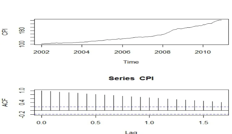
stable estimates of parameters. The order of integration of the series was
tested using seasonal unit root test. The result shows the annual unit root
of order 2 i.e. is integrated of order 2. The estimated models using SARIMA
Gen.jpeg
Figure 1: Time series and ACF plot of General CPI
4.2
Results and Discussion
The comparison using forecast accuracy measure is given in the following
table.
s In above table we can see that modeling CPI general using FTSA is
far far better than modeling using SARIMA. MSE shows FTSA is almost
7 times better than SARIMA. RMSE shows almost double efficiency over
SARIMA. MAE almost 3 times and MEDAE shows that forecast accuracy
of FTSA is 5 times better than SARIMA in modeling general CPI.
We can see that forecasted value using FTSA has less difference than
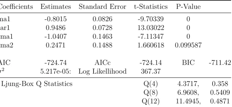
Table 2: SARIMA model of General CPI
Coefficients Estimates Standard Error t-Statistics P-Value
ma1 -0.8015 0.0826 -9.70339 0
sar1 0.9486 0.0728 13.03022 0
sma1 -1.0407 0.1463 -7.11347 0
sma2 0.2471 0.1488 1.660618 0.099587
AIC -724.74 AICc -724.14 BIC -711.42
σ2
5.217e-05: Log Likellihood 367.37
Ljung-Box Q Statistics Q(4) 4.3717, 0.358
Q(8) 6.9608, 0.5409
Q(12) 11.4945, 0.4871
FTSA over SARIMA models using data of general CPI. So modelling using
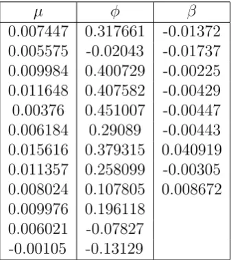
Table 3: FTSA estimated parameters µ, φ and β of CPI general
µ φ β
0.007447 0.317661 -0.01372 0.005575 -0.02043 -0.01737 0.009984 0.400729 -0.00225 0.011648 0.407582 -0.00429 0.00376 0.451007 -0.00447 0.006184 0.29089 -0.00443 0.015616 0.379315 0.040919 0.011357 0.258099 -0.00305 0.008024 0.107805 0.008672 0.009976 0.196118
0.006021 -0.07827 -0.00105 -0.13129
Table 4: Forecast accuracy comparison of General CPI
Method MSE RMSE MAE MEDAE
[image:28.595.146.452.376.422.2]