Munich Personal RePEc Archive
"Too big to fail" or "Too non-traditional
to fail"?: The determinants of banks’
systemic importance
Moore, Kyle and Zhou, Chen
Erasmus University Rotterdam, De Nederlandsche Bank
23 February 2013
Online at
https://mpra.ub.uni-muenchen.de/45589/
“Too big to fail” or “Too non-traditional to fail”?
The determinants of banks’ systemic importance
∗Kyle Moore
†Erasmus University Rotterdam and Tinbergen Institute
Chen Zhou
‡De Nederlandsche Bank and Erasmus University Rotterdam
March 25, 2013
Abstract This paper empirically analyzes the determinants of banks’ systemic importance. In constructing a measure on the systemic importance of financial insti-tutions we find that size is a leading determinant. This confirms the usual “Too big to fail” argument. Nevertheless, banks with size above a sufficiently high level have equal systemic importance. In addition to size, we find that the extent to which banks engage in non-traditional banking activities is also positively related to banks’ systemic importance. Therefore, in addition to “Too big to fail”, systemically important financial institutions can also be identified by a “Too non-traditional to fail” principle.
Keywords: Too-big-to-fail, systemic importance, systemic risk, non-traditional banking, extreme value theory
JEL Classification Numbers: G01, G21, G28
∗The research of Kyle Moore has received funding from the European Community’s Seventh
Frame-work Programme FP7-PEOPLE-ITN-2008. The funding is gratefully acknowledged. We are also grateful for the research assistance provided by Lin Zhao. Views expressed do not necessarily reflect official po-sitions of De Nederlandsche Bank.
†Email: [email protected]
1
Introduction
The failure of a single financial institution has the potential to spark catastrophic
losses in local, regional, and global financial systems. The global financial crisis which
unfolded in 2008 has provided an example. In order to prevent a potential meltdown of
the financial system, the US government was prompted to save large financial institutions
in the onset of this crisis. The intervention activities have lead to debates in support and
objection of rescuing certain distressed financial institutions. Arguments in favor stress
that financial institutions receiving government support are systemically important. That
is, their failure may trigger a relatively large number of simultaneous failures within
the financial sector. Nevertheless, the institutions that in practice receive most, if not
all, the “bailout” attention are large firms. In other words, although bailouts should
be conducted for “systemically important financial institutions” (SIFIs), the practical
principle is simply to rescue firms that are “Too big to fail” (TBTF). This suggests that
large financial institutions are automatically SIFIs. However, such an assertion requires
a careful empirical examination. This is the first question this paper addresses: Is size
fundamental in characterizing the systemic importance of a financial institution? If size
is not the sole determinant in differentiating banks’ systemic importance, the consequent
question is then: what are the other major bank-level characteristics that determine the
systemic importance of a financial institution? To answer these questions, this paper
empirically analyzes potential determinants of banks’ systemic importance.
In our framework, we distinguish the concept of systemic importance from “systemic
risk contribution”. The term “systemic risk” has been used in a number of different
contexts, and does not yet have a rigorous singular definition. It sometimes refers to
the system-wide risk in the financial sector1 and sometimes refers to the contribution
to the system-wide risk by one single institution.2 The former can be regarded as the
aggregation of the latter across all institutions in the system. Conceptually, systemic
1
Acharya et al. (2009) define systemic risk as “the risk of a crisis in the financial sector and its spill-over to the economy”.
2
risk contribution has two major components: the individual riskiness of the institution
and the spill-over effect to the rest of the system given its failure. Our definition of
the term systemic importance refers to the spill-over effect only. In this way, it reflects
the interconnectedness of the underlying institution to the rest of the system without
considering its own riskiness. This definition is consistent with the view of the Basel
Committee on Banking Supervision (BCBS) which stresses that “systemic importance
should be measured in terms of the impact that a failure of a bank can have on the global
financial system and wider economy rather than the risk that a failure can occur.”3
Our first major finding is that size is, to a large extent, able to differentiate systemic
importance; however, banks’ systemic importance is increasing in size only up to a certain
limit. For US banks during the crisis period (2007-2010), there is an increasing relation
between systemic importance and size only among those having total assets, at the end of
2006, below 30 billion USD.4 After this size “threshold” is surpassed, systemic importance
of banks remains stable. Hence, differentiating the systemic importance of banks by
only analyzing size is no longer possible. Furthermore, the cross-sectional dispersion on
systemic importance is also larger for smaller banks. Thus, it is necessary to investigate
other potential determinants for both large and small banks. With a close examination
of indicators on banks’ business models, our second major finding is that, in addition
to size, systemic importance is also determined by how much a bank relies on money
market funding to fund its projects and the amount of non-traditional income generating
activities a bank involves itself in. On the time dimension, our analysis on a selection of
US banks from the beginning of 1999 to the end of 2010 show that the determinants of
systemic importance are not invariant over time, but depend on changing macroeconomic
conditions. Lastly, we provide evidence that certain bank activities that serve to drive
systemic importance have an opposite effect on banks’ individual riskiness. Specifically,
banks that search out more non-traditional sources of funding and income generating
activities, generally have a lower individual risk at the expense of a greater systemic
3
See BCBS press release, “Global systemically important banks: Assessment methodology and the additional loss absorbency requirement”, November 2011.
4
importance.
One potential theoretical argument that supports “TBTF” is through bank
diver-sification. Large banks are usually better diversified compared to smaller banks. As
discussed in Wagner (2010), a well diversified bank bears less individual risks, while at
the same time, due to large common exposure, it is more systemically connected to the
rest of the system. Therefore, larger banks can be more systemically important. Such
a diversification argument can be well applied to other bank characteristics that are
po-tentially associated to systemic diversification. Particularly, engaging in non-traditional
banking activities such as generating non-interest profit and accessing interbank market
funding can be regarded as alternative methods for diversifying asset and funding risks,
thus may well be potential determinants of systemic importance.
Traditional banking that focuses on loan issuance and monitoring with interest income
are rather specialized. Although traditional banking may bear higher individual risk,
since different banks expose to different risk factors, the systemic linkage within the
system is low. With financial innovation, financial conglomerates engage in other
non-interest profit generating processes such as securitization or derivative trading. Such
banking activities increase diversification; at the same time, this diversification leads to
banks holding similar portfolios that are highly correlated. Consequently, this enhances
the possibility that financial institutions will suffer from common shocks to the asset
side of their balance sheets. This creates an indirect linkage in the event of a crisis,
see, e.g. de Vries (2005) and Acharya (2009). One step further, an initial shock on
bank asset value is likely to be amplified throughout the system as firms de-lever their
positions to meet margin calls and capital requirements (Brunnermeier and Pedersen
(2009)). Therefore, banks that engage more in activities generating non-interest profit
will be more systemically important. Two papers, De Jonghe (2010) and Knaup and
Wagner (2010), provide empirical evidence on the relation between non-interest income
and systemic risk. In De Jonghe (2010), the author finds that banks operating
non-traditional banking practices, such as reliance on commission and trading income, have
of funding. Knaup and Wagner (2010), while focusing on the asset decomposition on
banks balance sheets, find that non-traditional banking is more hazardous to the system
in terms of banks’ tail risk.
Another potential channel of systemic importance comes via non-traditional funding
such as interbank loans that take place in the money market. A great deal of the
lit-erature models systemic risk through the direct links banks expose themselves to each
other via the interbank markets, see, e.g. Rochet and Tirole (1996), Allen and Gale
(2000), and Freixas et al. (2000). The banking system is wired together as a network
supported by the interbank market. When banks have the ability and means to lend
to each other, it can be viewed as a diversified position to protect against liquidity risk:
liquidity constraints within the financial sector are reduced by introducing the interbank
market. Consequently, the financial system is able to absorb small to medium size
liquid-ity shocks. The downside of the interbank network is that banks open themselves up in
the event of a large liquidity shock which causes severe bank failure. The magnitude of a
banks exposure to the interbank market can therefore reflect the bank’s level of systemic
importance.
To summarize, if the diversification argument supports the statement of “TBTF”,
it should also support the statement that engaging in non-traditional banking activities
towards a more diversified position will enhance the systemic importance of a financial
institution. In other words, banks may well be “Too non-traditional to fail” (TNTTF).
As an empirical exercise, we test whether large bank size or high levels of engagement
in non-traditional banking are associated with high level of systemic importance. This
helps clarify whether TBTF or TNTTF should be the principle in identifying SIFIs.
For our empirical purpose, it is necessary to construct a measure on banks’ systemic
importance. Our proposed measure on systemic importance is based on the theoretical
interpretation that it pertains to the spill-over effect only. More specifically, it is defined
as the expected loss to the financial system given that one institution has failed. Thus,
we call our measure the “systemic loss given default” (SLGD). Given the failure of the
of expected losses of other institutions in the system. The systemic importance measures
derived thereof gives insight on the social welfare effects of a particular bank failure: it is
the liability the central authority faces if a particular bank fails and the other distressed
banks are not recapitalized. To measure these losses, we consider the potential loss on
insured deposits in the system given the failure of a specific financial institution. This
measure contributes to the literature on measuring systemic risk or systemic importance
of financial institutions.5 We differ from previous measures of systemic risk in two ways:
first, ours is a measure of systemic importance which does not contain information on
the individual riskiness of the underlying institution. Second, we consider a different
empirical strategy in estimating our proposed measure by implementing a multivariate
extreme value theory (EVT) approach.
As for measures on systemic importance, few studies have focused solely on the
spill-over effect. One candidate is the Shapley value, conceptualized in Tarashev et al. (2009).
Tarashev et al. (2010) applies the Shapley value concept to construct empirical measures
on systemic importance of individual institutions. Although intuitive in its interpretation,
the potential downside of the Shapley value is that it requires a large amount of calculation
which prohibits its empirical application to a large financial system. The other candidate
for measuring systemic importance is the Systemic Impact Index (SII) of Zhou (2010).
As we shall discuss in Section 2, our proposed SLGD measure is a generalization of the
SII measure which considers the economic impact to the system given the failure of one
single institution.
5
The paper proceeds as follows. We first propose a measure of systemic importance in
Section 2. Section 3 describes data and our empirical strategy on how we estimate the
systemic importance measure along with how we analyze the potential determinants of
systemic importance. The empirical results are reported in Section 4. Section 5 compares
the determinants of systemic importance with that of individual risk. Section 6 concludes
the paper and provides a discussion on possible policy implications.
2
Measuring Systemic Importance
Our measure on the systemic importance of one financial institution can be viewed
as a generalization of the systemic importance measure proposed by Zhou (2010), the
systemic impact index (SII). We start with reviewing the SII measure and discussing its
shortcoming.
The SII measure considers the expected number of simultaneous failures in the system
given the failure of one institution. Consequently, it is an aggregation of the conditional
probabilities of other banks’ failure given the failure of a specific bank. A direct
esti-mation of the probability of joint failure is difficult due to the scarcity of actual “bank
failures”. This issue has been resolved empirically by applying multivariate EVT.6
In-stead of estimating the conditional probability of joint failures, the EVT approach proxies
that by estimating conditional probability of joint bank distresses. A distress event is
described as the market price of a bank’s equity experiences a large loss. Evidence
sug-gests that financial market data, such as a bank’s market price of equity, can serve as an
early warning indicator of ratings changes for publicly traded bank holding companies
(BHCs), see, e.g. Krainer and Lopez (2003). Therefore, by considering the co-movement
of distress events, it provides a good proxy for the conditional probability of joint failure.
Consider a banking system consisting of N banks. Denote their equity returns as
X1, . . . , XN. A distress, or tail event, is defined as an event with a low probability p.7
In other words, values of Xi below a certain threshold level are assumed to trigger a
6
See De Haan and Ferreira (2006) for an overview of multivariate EVT.
7
tail event for bank i with probability p. Thus, this threshold level corresponds to the
Value-at-Risk (VaR) of the bank
P r(Xi <−V aRi(p)) =p, (2.1)
for some (tail) probability level p. While the choice of p is of concern for regulators
and the internal risk management of the firm, we do not impose a specific p level here.
Instead, we consider an equivalent p level across firms. Notice that this does not imply
that the threshold levels are identical across firms, but rather that the probability of a tail
event is invariant. Certain firms have a greater loss tolerance than others can thus enjoy
a lower threshold for defining a tail event. Such a description allows for heterogeneity in
banks’ individual risk taking activities.
The SII is then defined as
SIIi(p) =E(
X
j6=i
IXj<−V aRj(p)|Xi <−V aRi(p))
=X
j6=i
P(Xj <−V aRj(p)|Xi <−V aRi(p)), (2.2)
where IA is the indicator function that is equal to 1 if A occurs and 0 otherwise. If the
distress of one bank is likely to be accompanied by similar distresses in other banks, this
bank is said to be systemically important.8
From the definition, this measure is able to capture the general instability of the
sys-tem associated with the failure of a single institution. Although regulators may be
con-cerned with the number of failures in the system stemming from a single failure (Acharya
and Yorulmazer (2007)), such a measure lacks information on the exact economic impact
a failure would create. A distress in a bank which is accompanied by distress or failure
in other small banks, or a similar impact to large banks, are indistinguishable under this
8
This measure cannot discern any causality. For instance, a system consisting of only two banks has a correspondingSII1=SII2. Acharya (2009) argues that causality is not necessary in determining
measure. Hence, it is necessary to extend this measure to account for the economic size
of the impact.
Our proposed measure overcomes the shortcoming of the SII measure by considering
the real economic impact to the rest of the system given the failure of one bank. We
consider a measure of social welfare loss given distress to capture the systemic importance
of a bank as follows,
SLGD(p) = X
j6=i
LGDj ·P(Xj <−V aRj(p)|Xi <−V aRi(p)), (2.3)
where LGDj indicates the loss given default once bank j fails. The SII measure in Zhou
(2010) is then a special case in which LGDj = 1 across all firms.
Lastly, we choose a measure of loss, LGDj. During a period of economic turmoil,
when an acquisition of a failed bank by a competitor is not feasible, the government,
or monetary authority, is facing a decision of whether or not to rescue the bank from
bankruptcy using public funds. Considering that the authority decides, following the
failure of a bank, not to provide any bailout to the other banks that fail in conjunction.
As a consequence, they are responsible for the insured customer deposits held by the other
failed banks. Without having data on the specific size of insured deposits held by each
bank, we assume that the fraction of insured deposits against total customer deposits is
comparable across banks. We therefore use the amount of total customer deposits (DEP)
as a proxy for the amount of government insured deposits held by each bank. They act
as the weights used in constructing the SLGD measure of systemic importance.
3
Data and Methodology
3.1
Estimating the SLGD
The key element in estimating the SLGD measure, is the estimation of the conditional
probability that bankj fails given that bankifails for each pairiandj. For that purpose,
are collected from Datastream.9 We follow the approach in Hartmann et al. (2005) to
estimate such a conditional probability by applying multivariate EVT.
The multivariate EVT approach utilized in this paper improves upon existing
method-ology in the following way. Most existing measure of systemic risk use a statistical
methodology that assume multivariate normality. In contrast, there is a great deal of
empirical evidence to suggest that financial data follow a fat-tailed distribution as
op-posed to the normal distribution which tends to underestimate the probability of extreme
events, see, e.g. Mandelbrot (1963). Furthermore, the multivariate normal distribution
is known to exhibit tail independence, see, e.g. Sibuya (1959), while financial data have
non-negligible tail dependence. A methodology that incorporates a normality assumption
will underestimate the tail dependence.10 Lastly, to measure systemic risk or systemic
importance, the observations in the tail region are the only important observations that
should be considered in the estimation. Conversely, fitting data to the normal
distri-bution usually results in estimates which are determined by moderate level data. An
EVT approach allows for both heavy-tails and tail independence. It also focuses on the
observations in the tail region only while ignoring the observations at the moderate level.
Multivariate EVT provides models such that the limit of the conditional probability
is at a constant level as p→0, i.e.
τi,j := lim
p→0P(Xj <−V aRj(p)|Xi <−V aRi(p)). (3.1)
Thus, the conditional probability can be approximated by its limit τi,j. Suppose we have
n observations on the two return series as (Xi,s, Xj,s) for 1 ≤ s ≤ n. The limit τi,j can
be estimated by taking p = k/n for sample size n, where k := k(n) is an intermediate
9
Equities selected are traded on both the NYSE and the NASDAQ exchanges.
10
sequence such that k(n) → ∞ and k(n)/n → 0 as n → ∞. A non-parametric estimate
of τi,j is then given as
ˆ
τi,j :=
1
k
n
X
s=1
1Xj,s<Xj,(n−k),Xi,s<Xi,(n−k), (3.2)
where Xi,(n−k) is the (k+ 1)th lowest return amongXi,1, . . . , Xi,n.11
When estimating the conditional probabilities in the SII measure, Zhou (2010) uses
the raw equity returns to form the data set on (Xi,s, Xj,s). Such an approach does not
take into account the fact that the co-movement among bank equity returns can be
due to a common market factor. This may lead to an overestimation of the conditional
probabilities. In order to remove the dependence imposed by a common market factor, we
make correction by analyzing the banks excess returns over the market. We calculate the
residual equity returns over the market return12 by estimating the single-factor market
model in each estimation period as
Ri,s =αi+βiRm,s+ǫi,s. (3.3)
The error term,ǫi,s, is assumed to follow the standard assumptions of Ordinary Least
Squared (OLS) regression. The excess returns are calculated by
ˆ
ǫi,s=Ri,s−αˆi−βˆiRm,s. (3.4)
We use the estimated excess returns (ˆǫi,s,ˆǫj,s) instead of raw returns as the data set
on (Xi,s, Xj,s) in the estimation of the conditional probabilities.
Another technical issue in the estimation is the sequence choice of the intermediate
k in (3.2). The theoretical conditions on k are not relevant for a finite sample analysis.
Instead of taking an arbitrary k, a usual procedure is to calculate the estimator of τi,j
under differentk values and draw a line-plot of the estimates against thek values. With
11
For the estimator ofτi,j, usual statistical properties, such as consistency and asymptotic normality, has been proved, see, e.g. De Haan and Ferreira (2006).
12
a lowk value, the estimation exhibits a large variance, while for a high k value, since the
estimation uses too many observations from the moderate level, it bears a potential bias.
Therefore,k is usually chosen by picking the first stable part of the line-plot starting from
lowk, which balances the tradeoff between the variance and the bias. The estimates then
follow from such a choice of k. Because k is chosen from a stable part of the line-plot,
a small variation of the k value does not change the estimated value. Thus, the exactk
value is not sensitive for the estimation ofτi,j. In our empirical application, the chosenk
value differs for different pairs of banks, because the sample sizen, the number of available
excess returns in a given period, differs for different pairs of banks. Nevertheless, we keep
the ration k/n constant across different samples at a level of 3%.
We also impose a cutoff value, 0.10, in the estimation of τ-measure, such that values
of the estimated τ below the cutoff level are set to zero. This is to avoid the potential
positive bias in the estimation ofτ: when the actualτ value is zero, the estimation usually
yields a small positive value. Our regression results are robust for different selection of
cutoff values.
In addition to the conditional probabilities, the other element in the SLGD measure
is the calculation of loss given default. For that purpose we collect annual balance sheet
data on total customer deposits for each bank from the Bankscope database.13 Since
each estimation period covers four years, we use average total customer deposits over the
same period as the weights. With estimating the conditional probability for each pair of
banks iandj, the SLGD measure for bank iis then calculated as the sum of the product
of the conditional probabilities across all other banks, j 6=i, and bank j’s total customer
deposits.
3.2
Analyzing Potential Determinants
To analyze the potential determinants of systemic importance, we collect bank balance
sheet data, construct indicators reflecting their business models and perform regression
analysis between the SLGD measure and the indicators. The size of the bank, our primary
13
focus, is measured as the logarithm of total assets in millions of USD. To capture a possible
non-linear property of the size, we also consider its quadratic form in regressions. In
order to avoid a potential multi-collinearity issue, the size is first standardized by its
cross-sectional mean and standard deviation and then squared.
The focus on non-traditional banking activities is implemented by considering the
following variables: money market funding as a ratio of total funding and non-interest
income as a ratio of total income. The latter variable is further decomposed into two
variables representing trading income and fee and commission income both as a ratio of
total income.
Five control variables based on the CAMEL rating system14 are included in the
re-gressions as follows:
• Capital adequacy: Tier 1 Capital Ratio
• Asset quality: Gross Loans/ Total Assets
• Management: Problem Loans/ Total Loans
• Earnings: Return on Average Assets
• Liquidity: Liquid Assets/ Short-term Funding
We conduct our regression analysis in two ways. First, we analyze only the period
between 2007 and 2010 which encapsulates the financial crisis. The choice of having a
four year period for our analysis is to ensure a sufficient number of observations for the
estimation of the conditional probabilities used in the SLGD measure. We filter out any
institution that is not traded on at least 80% of the days within this period. We match
the estimated SLGD measure with the annual balance sheet data recorded at the end of
the year in 2006. After this filtering procedure, 311 BHCs are included in our regression
analysis. Since the business model indicators are ahead of the SLGD measure in time,
14
our regression analysis forms an out-of-sample, or forward-looking approach. This allows
analyzing the relation between the business model of a bank before the financial crisis
and its systemic importance during the crisis.
Second, in order to see whether the drivers of systemic importance stand over a longer
time horizon, we extend our analysis to cover a period from the beginning of 1999 to the
end of 2010. Under this approach, the SLGD measure is estimated in the same way over
each four-year period that is rolled forward year by year in the sample, i.e. the SLGD
measures are estimated for the periods 1999-2002, 2000-2003, ..., 2007-2010. We removed
any bank that was not traded on at least 90% of the days covering the whole period and
did not have end-of-year balance sheet data from 1998 to 2007. This filtering process
results in a panel data set consisting of 143 banks over 8 estimation periods. With the
1125 firm-period observations in total, we perform a panel regression with time fixed
effects while clustering at the bank level.
Lastly, we split the panel data set to perform eight separate OLS regressions, one for
each period, in the same way as for the crisis period. This allows us to check how the
determinants have emerged over the entire time horizon.
4
Empirical Results
4.1
Financial Crisis: 2007-2010
Our main result is conducted over the most recent period in our data set (2007-2010),
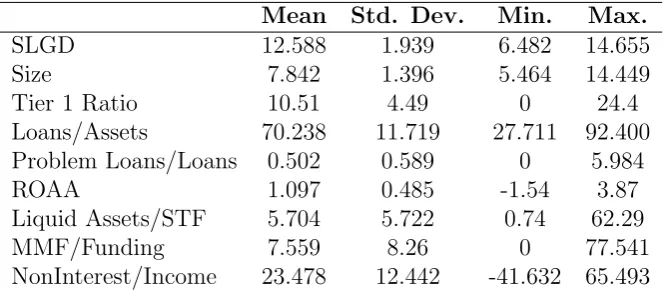
which manifests the time surrounding the financial crisis. Table 1 provides descriptive
statistics of the SLGD and potential determinants. Table 2 shows the correlation among
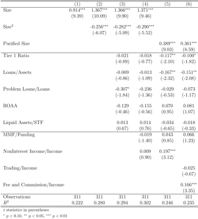
the potential determinants. Table 3 reports the regression results.
The first regression (column 1) only contains one independent variable: the size of
banks. It is positive and significant at the 99% confidence level. This result gives support
to the TBTF argument that larger banks are more systemically important. We then take
a close look at size in the second regression (column 2) by adding the quadratic form of
the 99% level, the quadratic term is negative and significant at the same confidence level.
Hence, the relation between the SLGD and size is non-linear.
In order to have a better insight on the non-linearity, we further analyze the quadratic
relation between SLGD and Size as
SLGD=aSize2+bSize+c.
By taking the first-order derivative, we get that ∂SLGD
∂Size = 2aSize + b. Hence, for
Size=−b
2a, the partial derivative turns to be zero. In other words, the SLGD is neither
increasing nor decreasing with respect to the variation of Size at such a level. With the
estimation of the coefficients a and b as in Table 3 (column 2), we find that this occurs
at Size = 11.5.15 By partitioning the sample into two groups at Size= 11.5, we find a
significantly positive relationship for banks with Size < 11.5, while for Size ≥ 11.5 we
find a slope coefficient that is indistinguishable from zero at the 95% confidence level. In
other words, the SLGD of banks increase with respect to the size up to a certain threshold
and then no further. This observation implies that for large banks with Size≥11.5 the
TBTF principle does not hold. Since the cutoff point 11.5 is rather close to the
maxi-mum size in the sample, the quadratic relation, in fact, would be better characterized as
a “kink” relation. We attempt to identify the size level where the insignificance of the
SLGD−Sizerelation starts.
Starting at 11.5 and decreasing the threshold, the regression based on large banks
remains insignificant until the threshold level reaches 10.3. When splitting the sample at
Size= 10.3, the SLGD is strictly increasing in size whenSize <10.3 and the regression
coefficient for size is insignificant at the 95% confidence level forSize≥10.3. Below this
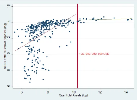
size threshold the SLGD−Size relation is positive. This relation is shown graphically
in a scatter plot of SLGD against Size in Figure 1.16
15
TheSizeand Size2
term are constructed from standardized variables in order to remove the po-tential multi-collinearity problem. as a result, the solution to the above equation had to be transformed back to the original size using the transformationSizeσ+µ.
16
Alternatively, we can run a threshold regression to search for a breakpoint that partitions the sample of banks into two segments. We utilize a test from Hansen (1999) and find a breakpoint, significant at the 95% confidence level, to be atSize= 9.4. This is close to the 10.3 cutoff point of theSLGD−Size
Our empirical analysis confirms that large banks are systemically important, but only
after a certain size level is reached. This level corresponds to a bank with total assets
equaling or exceeding roughly 30 billion USD. After this threshold is surpassed, size
alone cannot differentiate between the degree of systemic importance among those large
US banks. This finding partially supports the validity of the TBTF argument.
To further analyze determinants of systemic importance, we add other control
vari-ables, i.e. the CAMEL ratios, to the regression alongsideSize. The regression results on
Sizeand its quadratic term remain unchanged. This remains the case when the variables
representing non-traditional banking are added to the regression. Hence the non-linear
size-systemic importance relation is rather robust.
We further test the TNTTF argument by performing regressions with the variables
indicating non-traditional banking. In the regression including the level and quadratic size
variables (column 4) none of the variables on non-traditional banking are significant at
even the 90% confidence level. This may well be a consequence of a potential endogeneity
problem. When considering both size and other variables indicating a bank’s business
model, size is endogenous if the strategies and activities a bank chooses to undertake have
direct impact on how large the bank becomes. Thus, the bank size is endogenously related
with other variables including the variables describing non-traditional banking activities.
Table 2 shows the correlation matrix among the size variable and other variables used in
the analysis. A high correlation is observed, especially between size and variables on
non-traditional banking. This could potentially overwhelm the size effect or shield any possible
effects that other variables may contribute in determining a bank’s systemic importance.
In order to avoid such a problem, we orthogonalize the size variable by first regressing
it against the other variables in the regression and then taking the residual term as a
“purified size” variable. By including the purified size variable, the estimated coefficients
on other variables in the regression will indicate their own contribution towards systemic
importance independent of the bank size.
When we replace the size variable and its quadratic form with the purified size in
the regression, the purified size variable is positive and significant, while the non-interest
income variable is also positive and significant at the 99% level. Therefore, we conclude
that the non-interest income activities of a bank play a role in determining a bank’s
systemic importance. This supports the theoretical argument that as banks move from
more traditional activities (e.g. deposit taking and lending) towards more non-traditional
sources of income they increase their systemic connectedness (Shleifer and Vishny (2010)).
This result is also consistent with the empirical finding in Brunnermeier et al. (2011).
By further dividing the non-interest income variable into two variables indicating trading
income and fee and commission income both as a ratio of total income, we observe that the
contribution of non-interest income to systemic importance is determined by the amount
of fee and commission income that a bank undertakes while the amount of trading income
does not appear to be significant. For the funding side, we find the money market funding
variable to be positive, yet insignificant at the 90% confidence level.
In addition to the positive effect of non-interest income on systemic importance, we
also find that among the CAMEL ratios, the amount of Tier 1 capital a bank holds in
relation to its risk-weighted assets and the fraction of assets that are made up of loans
both contribute negatively to a bank’s systemic importance level. Banks with a larger
capital buffer prior to the crisis and with a greater focus on more traditional banking
activities (e.g. issuing loans), are less connected to the system during the crisis.
From these results, we have evidence that SIFIs, in addition to being identified by the
TBTF principle, also have the potential of being TNTTF. Here non-traditional refers to
relying heavily on non-interest income generating activities in the form of fee and
com-mission income. Further, a bank operating in a more traditional manner of maintaining a
healthy capital buffer and engaging in loan issuing activities corresponds to a lower level
4.2
Multi-period Analysis
To check if the results of our analysis during the crisis period are robust for periods
outside the crisis, we extend our sample of data to a larger horizon starting from the
beginning of 1999 to the end of 2010. As depicted in Section 3.2, the data set includes
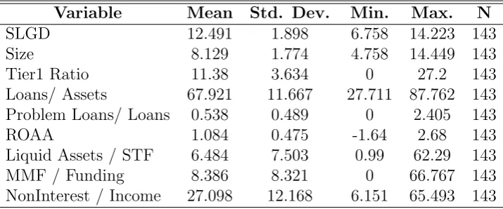
eight overlapping estimation periods. Table 5 provides descriptive statistics of the SLGD
and potential determinants. The results of the panel regression over this time period are
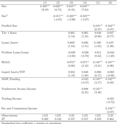
shown in Table 4.
In the panel regression we again find that bank size has a non-linear effect on its
systemic importance: a positive and significant coefficient on the size variable while a
negative and significant coefficient on the quadratic size term. The point estimates are
close to the ones found in the 2007-2010 estimation period which hints that a potential
“kink” relation remains. Furthermore, the purified size also remains significant at the
99% confidence level. To summarize, the overall effect of size on systemic importance is
robust over an extended time period and smaller sample of banks.
Of the variables indicating non-traditional banking, the non-interest income ratio
remains significant at the 99% confidence level. However, a key difference is that the
coefficient on the money market funding variable is now also significant and positive at
the 99% confidence level. The new result agrees with the theoretical argument that a
shift away from traditional funding (e.g. deposit taking) towards more non-traditional
funding sources was instrumental in the cause of the crisis due to their susceptibility to
runs, see, e.g. Acharya, Gale and Yorulmazer (2010). The fact that we did not observe
such a strong significance of the money market funding variable in the regression during
the crisis period is potentially due to sample selection. In the single period exercise, our
sample contains a large amount of banks that actually undertook a limited amount of
money market funding. By having a lower amount of banks in the panel data analysis,
the sample selection procedure results in selecting more large banks that have extensively
accessed the money market funding. Money market funding now appears as a strong
determinant of bank systemic importance among those selected banks.
in coefficients of the determinants of systemic importance over time. We thus analyze
each of the eight estimation periods separately, which allows the potential evolution of
determinants across a changing macroeconomic climate.
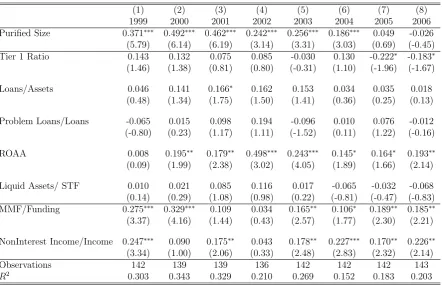
Table 6 shows the regression results for each of the eight estimation periods. The
general observation is that the determinants are varying over time. First, the purified
size is a strong positive determinant of systemic importance over the first six periods,
but this relation disappears in the final two periods. The result in the last period does
not necessarily contrast with that in our single period analysis with the larger sample of
banks. The sample selection procedure leading to this new result removed many small
banks since they did not survive over the period 1999-2010. Hence, the remaining banks
are, in general, large. This is confirmed in Table 5 with summary statistics. Therefore,
the new results simply reflect the non-significant effect among large banks found in the
previous single period regression.
Of the variables on non-traditional banking, the non-interest income is positive and
significant in six of the eight periods including not only all periods covering the
finan-cial crisis and the dot-com collapse, but also one of the periods under more benign
economic conditions between the two downturns. Hence, the positive relation between
non-traditional sources of income and systemic importance is robust for both an extended
time period and over different macroeconomic conditions. This gives support in favor of
the TNTTF principle over the TBTF principle in identifying SIFIs: it holds during both
positive and negative economic conditions. The money market funding variable is
pos-itive and significant at the 95% confidence level for most of the periods with the only
exceptions being the two neighboring periods of 2002-2005 and 2003-2006. The two
peri-ods cover the booming macroeconomic climate between the dot-com bubble collapse and
the financial crisis, whereas the other six periods contain, at least to some extent, a time
during an economic downturn or crisis. Our results provide evidence that a reliance on
money market funding plays a prominent role in determining the systemic importance of
banks during times of economic distress. This again supports the notion that banks are
5
Determinants of Individual Risk: A Comparison
We compare the determinants of banks’ systemic importance with that of a banks’
individual risk. We have shown that certain banking characteristics determine banks’
systemic importance, namely the size and levels of bank’s non-traditional activities. As
a measure of systemic importance, the SLGD measure is constructed in such a way that
it is independent of bank’s individual risk. Nevertheless, conceptually, the individual
risk and the systemic importance are the two components of systemic risk of a financial
institution. Thus, when attempting to mitigate systemic risk, in addition to identifying
the determinants of systemic importance, it is necessary to check the relation between
individual risk and the bank’s business model.
The individual risk of a bank is measured from the same equity price data that we
used in the construction of the SLGD measure. We consider the heavy-tailed feature of
equity returns by employing univariate EVT to calculate each banks expected shortfall
(ES) on its equity returns. The heavy-tailedness of financial returns is well-documented
in literature, see e.g. Jansen and de Vries (1991) and Embrechts et al. (1997). It shows
that a power law fits the downside tail distribution of the equity return Xi,
P(Xi <−u)∼Aiu−αi as u→+∞. (5.1)
Here, the parameters αi is the so-called tail index. From such a parametric expansion of
the tail distribution, it follows that, if αi >1,
ESi(p) :=−E(Xi|Xi <−V aRi(p))∼
αi
αi−1
V aRi(p) as p→0. (5.2)
Similar to the estimation of τi,j, the V aRi(p) at the level p = k/n is estimated by
the (k+ 1)th highest losses, −Xi,(n−k), where Xi,(n−k) is the (k+ 1) lowest return. The
estimation of αi is achieved by way of the Hill estimator from univariate EVT. With
is defined as
1/αˆi :=
1
k
k
X
i=1
log(−Xi,(n−i+1))−log(−Xi,(n−k)). (5.3)
For the statistical properties of the Hill estimator, see Hill (1975). With the estimation
of the V aR and the tail index, we obtain the estimate of the ES on the return series
of each bank. In other words, we have eight overlapping periods during which the ES
of each bank is measured. We use these estimates to run a panel regression against the
bank business model indicators in the same way as for the SLGD measure, using time
fixed effects and clustering at the bank level.
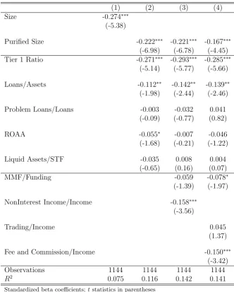
Table 7 reports the results of the regressions. First, we regress the ES against only the
Sizevariable and find it to be negative and significant at the 99% confidence level (column
1). This is consistent with theoretical literature that larger banks are less risky due to
diversification. For the regressions involving the CAMEL ratios and the variables on
non-traditional banking, we use the purified size variable to avoid any potential endogeniety.
The variable for non-interest income is negative and significant at the 99% confidence
level. By decomposing this variable into trading income and fee and commission income
(column 4), we find that the coefficient for fee and commission income variable is negative
and significant at the 99% confidence level while that for trading income is insignificant. In
the regression where with the decomposition of the non-interest income, we also find that
the variable on money market funding is negative and significant at the 90% confidence
level. All of these findings provide evidence that engaging in non-traditional banking
reduces the individual risk a bank faces.
Among the CAMEL ratios, the amount of Tier 1 capital and loans as a fraction of
total assets are negative and significant at the 99% and 95% confidence levels, respectively.
The returns on assets variable is negative but only significant at the 90% confidence level
when excluding the variables on non-traditional activities (column 2). These results show
that more capitalized banks have lower individual risk. Banks that engage mainly in loan
issuance are also less risky. The latter a potential consequence of the fact that our data
set covers the period of the housing bubble, during which traditional loan activity was
To summarize, we find that the determinants of systemic importance, size and
non-traditional banking, induce an opposite effect on the individual risk of a bank. A potential
explanation is through the diversification effect. Banks can limit their own individual
risk of failure by diversifying their activities. This is accomplished by extending the
scope of business activities as well as engaging in non-traditional banking activities. At
the same time, these actions increase commonalities between banks which lead to an
increased systemic importance. Determinants of the individual risk and the systemic
importance may thus work against one another. In other words, by being involved with
non-traditional banking, banks shift their individual risk to the system by enhancing their
systemic importance.
6
Conclusion
This paper addresses the question of whether the size of a financial institution is
fundamental in characterizing its systemic importance. In other words, can we identify
SIFIs following the TBTF principle? We find partial support in favor of the TBTF
hypothesis; however, the relation between size and systemic importance is non-linear.
More specifically, systemic importance is positively related to size only up to a certain
limit. For example, as of the end of 2006, US banks with total assets exceeding 30 billion
USD are equally systemically important during the crisis period (2007-2010). Hence,
systemic importance cannot be differentiated by analyzing size only.
Upon further examination, we find that systemic importance is also determined by the
extent to which a bank engages in non-traditional activities. The systemic importance of
financial institutions is positively related to both the amount of funding from the money
market and the income generated from non-interest activities, in particular, the fee and
commission income. Furthermore, banks which operate under a traditional manner such
as holding a high level of Tier 1 capital and relying on loan issuing activities have a lower
systemic importance.
we show that the determinants of systemic importance are not time invariant. While
the size of a bank is a strong indicator of its systemic importance before the global
financial crisis, non-traditional banking activities are predominant in periods of economic
downturn or crisis. Finally, we find that the determinants of systemic importance may
have an opposite effect on the individual riskiness of banks. In other words, banks that
diversify their positions in order to reduce individual risk may at the same time increase
their systemic importance.
Our empirical findings have direct policy implications for regulators. First, regulation
that attempts to reduce systemic risk in a financial system must take into account the
size of financial institutions, but only to a limited degree. Once banks become sufficiently
large, their systemic importance can no longer be differentiated by size. In that case, the
systemic impact that large banks have on the system has to be differentiated by analyzing
other bank characteristics. More specifically, non-traditional banking activities such as
engaging in non-interest profit generating activities or using money market funding can
also lead a bank to be a SIFI. Second, macro-prudential regulation that varies according
to the macroeconomic environment is necessary to maintain the stability of the system.
We observe the time variation of the potential determinants for systemic importance,
which indicates that regulation has to vary with the business cycle. “Flat” regulation
that does not consider macroeconomic environment may provide a sub-optimal solution.
Third, when attempting to mitigate the risk taking behavior of financial institutions, it
is important to be aware of the potential increase in its spill-over effects to the rest of the
system. The interaction between the two sources of systemic risk shows a potential
trade-off between mitigating individual risk and amplifying interconnectedness. Understanding
the drivers of the two components of systemic risk is the first step in designing effective
References
Acharya, V. (2009), ‘A theory of systemic risk and design of prudential bank regulation’,
Journal of Financial Stability 5(3), 224–255.
Acharya, V., Brownlees, C., Engle, R., Farazmand, F. and Richardson, M. (2010),
Mea-suring systemic risk, Wiley Online Library.
Acharya, V., Gale, D. and Yorulmazer, T. (2010), Rollover risk and market freezes,
Technical report, National Bureau of Economic Research.
Acharya, V., Pedersen, L., Philippon, T. and Richardson, M. (2009), ‘Regulating systemic
risk’,Chapter 13: ”Restoring financial stability: How to repair a failed system”, John
Wiley Sons pp. 283–304.
Acharya, V. and Yorulmazer, T. (2007), ‘Too many to fail–an analysis of
time-inconsistency in bank closure policies’,Journal of Financial Intermediation16(1), 1–31.
Adrian, T. and Brunnermeier, M. (2011), Covar, Technical report, National Bureau of
Economic Research.
Allen, F. and Gale, D. (2000), ‘Financial contagion’, Journal of Political Economy
108(1), 1–33.
Brunnermeier, M., Dong, G. and Palia, D. (2011), ‘Banks non-interest income and
sys-temic risk’, Princeton University and Rutgers University .
Brunnermeier, M. and Pedersen, L. (2009), ‘Market liquidity and funding liquidity’,
Re-view of Financial Studies 22(6), 2201–2238.
De Bandt, O. and Hartmann, P. (2000), ‘Systemic risk: A survey’, ECB Working Paper
No. 35.
De Haan, L. and Ferreira, A. (2006), Extreme value theory: An introduction, Springer
De Jonghe, O. (2010), ‘Back to the basics in banking? a micro-analysis of banking system
stability’, Journal of Financial Intermediation19(3), 387–417.
de Vries, C. (2005), ‘The simple economics of bank fragility’, Journal of Banking &
Finance29(4), 803–825.
Embrechts, P., Kl¨uppelberg, C. and Mikosch, T. (1997), Modelling extremal events for
insurance and finance, Springer Verlag.
Freixas, X., Parigi, B. and Rochet, J. (2000), ‘Systemic risk, interbank relations, and
liquidity provision by the central bank’,Journal of Money, Credit and Bankingpp. 611–
638.
Hansen, B. (1999), ‘Threshold effects in non-dynamic panels: Estimation, testing, and
inference’,Journal of Econometrics 93(2), 345–368.
Hartmann, P., Straetmans, S. and De Vries, C. G. (2005), Banking system stability: A
cross-atlantic perspective, Technical report, National Bureau of Economic Research.
Hill, B. (1975), ‘A simple general approach to inference about the tail of a distribution’,
The Annals of Statistics pp. 1163–1174.
Hirtle, B. and Lopez, J. (1999), ‘Supervisory information and the frequency of bank
examinations’,Economic Policy Review 5(1).
Huang, X., Zhou, H. and Zhu, H. (2010), ‘Systemic risk contributions’, Journal of
Fi-nancial Services Research pp. 1–29.
Jansen, D. and de Vries, C. (1991), ‘On the frequency of large stock returns: Putting
booms and busts into perspective’,The Review of Economics and Statisticspp. 18–24.
Knaup, M. and Wagner, W. (2010), Measuring the tail risks of banks, Technical report,
NCCR Working paper, NCCR.
Krainer, J. and Lopez, J. (2003), ‘How might financial market information be used for
su-pervisory purposes?’,Economic Review-Federal Reserve Bank of San Franciscopp. 29–
Mandelbrot, B. (1963), ‘The variation of certain speculative prices’, The journal of
busi-ness 36(4), 394–419.
Rochet, J. and Tirole, J. (1996), ‘Interbank lending and systemic risk’,Journal of Money,
Credit and Banking 28(4), 733–762.
Segoviano, M. and Goodhart, C. (2009), Banking stability measures, International
Mon-etary Fund.
Shleifer, A. and Vishny, R. (2010), ‘Unstable banking’, Journal of Financial Economics
97(3), 306–318.
Sibuya, M. (1959), ‘Bivariate extreme statistics, i’, Annals of the Institute of Statistical
Mathematics 11(2), 195–210.
Tarashev, N., Borio, C. and Tsatsaronis, K. (2009), ‘The systemic importance of financial
institutions’,BIS Quarterly Review 75, 87.
Tarashev, N., Borio, C., Tsatsaronis, K., for International Settlements. Monetary, B. and
Dept, E. (2010),Attributing systemic risk to individual institutions, number 308, Bank
for International Settlements.
Wagner, W. (2010), ‘Diversification at financial institutions and systemic crises’, Journal
of Financial Intermediation 19(3), 373–386.
Zhou, C. (2010), ‘Are banks too big to fail? measuring systemic importance of financial
7
Tables and Figures
Table 1: Summary Statistics: SLGD (2007-2010) and potential determinants (2006)
Mean Std. Dev. Min. Max.
SLGD 12.588 1.939 6.482 14.655
Size 7.842 1.396 5.464 14.449
Tier 1 Ratio 10.51 4.49 0 24.4
Loans/Assets 70.238 11.719 27.711 92.400
Problem Loans/Loans 0.502 0.589 0 5.984
ROAA 1.097 0.485 -1.54 3.87
Liquid Assets/STF 5.704 5.722 0.74 62.29
MMF/Funding 7.559 8.26 0 77.541
NonInterest/Income 23.478 12.442 -41.632 65.493
Table 2: Correlation: Determinants of Systemic Importance (2006)
Variables Size Tier 1 Ratio Loans/Assets Problem/Loans ROAA Liquid/STF MMF NonInterest
Size 1.000
Tier 1 Ratio -0.089 1.000
Loans/Assets -0.270 -0.206 1.000
Problem/Loans 0.005 0.039 -0.049 1.000
ROAA 0.181 0.160 0.172 -0.284 1.000
Liquid/STF 0.375 -0.045 -0.335 0.069 0.108 1.000
MMF 0.359 0.104 -0.419 0.178 -0.055 0.227 1.000
NonInterest 0.454 -0.051 -0.184 -0.172 0.174 0.237 0.137 1.000
Note: This table presents the correlation matrix among the potential determinants of systemic importance. The size refers to the total assets of a bank in (log) million USD. The Tier 1 Ratio is the total Tier 1 capital divided by the bank’s risk-weighted assets. The loans to asset ratio is calculated as the gross loans of a bank divided by its total assets. The problem loans ratio is the total non-performing loans divided by the gross loans of the bank. The ROAA variable is the return on average assets. The Liquid Assets/STF is calculated at the amount of liquid assets a bank holds divided by the amount of short-term funding the bank has acquired. MMF/Funding is calculated as the total money market funding divided by total funding. NonInterest/Income is calculated as the amount of non-interest income as a ratio of total income.
Table 3: The Determinants of Systemic Importance: 2007-2010
(1) (2) (3) (4) (5) (6)
Size 0.914∗∗∗ 1.367∗∗∗ 1.366∗∗∗ 1.371∗∗∗
(9.39) (10.09) (9.90) (9.46)
Size2 -0.256∗∗∗ -0.282∗∗∗ -0.290∗∗∗
(-6.07) (-5.09) (-5.52)
Purified Size 0.389∗∗∗ 0.361∗∗∗
(9.03) (8.59)
Tier 1 Ratio -0.021 -0.018 -0.117∗∗ -0.100∗
(-0.89) (-0.77) (-2.10) (-1.82)
Loans/Assets -0.009 -0.013 -0.167∗∗ -0.151∗∗
(-0.86) (-1.09) (-2.32) (-2.08)
Problem Loans/Loans -0.307∗ -0.236 -0.029 -0.073
(-1.84) (-1.36) (-0.53) (-1.17)
ROAA -0.129 -0.155 0.070 0.081
(-0.46) (-0.56) (0.95) (1.07)
Liquid Assets/STF 0.013 0.014 -0.034 -0.018
(0.67) (0.76) (-0.65) (-0.33)
MMF/Funding -0.019 0.043 0.066
(-1.40) (0.85) (1.23)
NonInterest Income/Income 0.009 0.197∗∗∗
(0.90) (3.12)
Trading/Income -0.025
(-0.67)
Fee and Commission/Income 0.166∗∗∗
(3.35)
Observations 311 311 311 311 311 311
R2 0.222 0.280 0.294 0.302 0.246 0.235
tstatistics in parentheses
∗p <0.10,∗∗p <0.05,∗∗∗p <0.01
Figure 1: SLGD vs. Size: 2007-2010.
Table 4: The Determinants of Systemic Importance: Panel Regression
(1) (2) (3) (4) (5) (6)
Size 0.403∗∗∗ 0.620∗∗∗ 0.610∗∗∗ 0.616∗∗∗
(9.19) (8.74) (8.45) (7.64)
Size2 -0.311∗∗∗ -0.323∗∗∗ -0.324∗∗∗
(-4.85) (-3.99) (-4.07)
Purified Size 0.218∗∗∗ 0.162∗∗∗
(6.37) (4.87)
Tier 1 Ratio 0.065 0.065 0.040 0.037
(1.54) (1.55) (0.80) (0.77)
Loans/Assets 0.088∗ 0.080 0.108∗ 0.105∗
(1.85) (1.51) (1.85) (1.86)
Problem Loans/Loans -0.029 -0.026 0.011 -0.043
(-0.83) (-0.70) (0.42) (-1.20)
ROAA 0.072∗∗ 0.071∗∗ 0.140∗∗∗ 0.167∗∗∗
(2.60) (2.42) (3.21) (4.96)
Liquid Assets/STF 0.052 0.048 0.006 -0.002
(1.19) (1.08) (0.17) (-0.06)
MMF/Funding -0.021 0.150∗∗∗ 0.162∗∗∗
(-0.47) (4.17) (4.68)
NonInterest Income/Income 0.008 0.135∗∗∗
(0.25) (3.46)
Trading/Income -0.021
(-0.72)
Fee and Commission/Income 0.158∗∗∗
(4.07)
Observations 1125 1125 1125 1125 1125 1125
R2 0.492 0.542 0.557 0.557 0.459 0.464
Standardized beta coefficients;tstatistics in parentheses
∗p <0.10,∗∗p <0.05,∗∗∗p <0.01
Table 5: Summary statistics: SLGD (2000-2010) and potential determinants
Variable Mean Std. Dev. Min. Max. N
SLGD 12.491 1.898 6.758 14.223 143
Size 8.129 1.774 4.758 14.449 143
Tier1 Ratio 11.38 3.634 0 27.2 143
Loans/ Assets 67.921 11.667 27.711 87.762 143
Problem Loans/ Loans 0.538 0.489 0 2.405 143
ROAA 1.084 0.475 -1.64 2.68 143
Liquid Assets / STF 6.484 7.503 0.99 62.29 143
MMF / Funding 8.386 8.321 0 66.767 143
NonInterest / Income 27.098 12.168 6.151 65.493 143
Table 6: The Determinants of Systemic Importance: 2000-2010
(1) (2) (3) (4) (5) (6) (7) (8)
1999 2000 2001 2002 2003 2004 2005 2006
Purified Size 0.371∗∗∗ 0.492∗∗∗ 0.462∗∗∗ 0.242∗∗∗ 0.256∗∗∗ 0.186∗∗∗ 0.049 -0.026
(5.79) (6.14) (6.19) (3.14) (3.31) (3.03) (0.69) (-0.45)
Tier 1 Ratio 0.143 0.132 0.075 0.085 -0.030 0.130 -0.222∗ -0.183∗
(1.46) (1.38) (0.81) (0.80) (-0.31) (1.10) (-1.96) (-1.67)
Loans/Assets 0.046 0.141 0.166∗ 0.162 0.153 0.034 0.035 0.018
(0.48) (1.34) (1.75) (1.50) (1.41) (0.36) (0.25) (0.13)
Problem Loans/Loans -0.065 0.015 0.098 0.194 -0.096 0.010 0.076 -0.012
(-0.80) (0.23) (1.17) (1.11) (-1.52) (0.11) (1.22) (-0.16)
ROAA 0.008 0.195∗∗ 0.179∗∗ 0.498∗∗∗ 0.243∗∗∗ 0.145∗ 0.164∗ 0.193∗∗
(0.09) (1.99) (2.38) (3.02) (4.05) (1.89) (1.66) (2.14)
Liquid Assets/ STF 0.010 0.021 0.085 0.116 0.017 -0.065 -0.032 -0.068
(0.14) (0.29) (1.08) (0.98) (0.22) (-0.81) (-0.47) (-0.83)
MMF/Funding 0.275∗∗∗ 0.329∗∗∗ 0.109 0.034 0.165∗∗ 0.106∗ 0.189∗∗ 0.185∗∗
(3.37) (4.16) (1.44) (0.43) (2.57) (1.77) (2.30) (2.21)
NonInterest Income/Income 0.247∗∗∗ 0.090 0.175∗∗ 0.043 0.178∗∗ 0.227∗∗∗ 0.170∗∗ 0.226∗∗
(3.34) (1.00) (2.06) (0.33) (2.48) (2.83) (2.32) (2.14)
Observations 142 139 139 136 142 142 142 143
R2 0.303 0.343 0.329 0.210 0.269 0.152 0.183 0.203
Standardized beta coefficients;tstatistics in parentheses
∗p <0.10,∗∗p <0.05,∗∗∗p <0.01
Table 7: The Determinants of Bank Individual Risk: Panel Regression
(1) (2) (3) (4)
Size -0.274∗∗∗
(-5.38)
Purified Size -0.222∗∗∗ -0.221∗∗∗ -0.167∗∗∗
(-6.98) (-6.78) (-4.45) Tier 1 Ratio -0.271∗∗∗ -0.293∗∗∗ -0.285∗∗∗
(-5.14) (-5.77) (-5.66)
Loans/Assets -0.112∗∗ -0.142∗∗ -0.139∗∗
(-1.98) (-2.44) (-2.46)
Problem Loans/Loans -0.003 -0.032 0.041 (-0.09) (-0.77) (0.82)
ROAA -0.055∗ -0.007 -0.046
(-1.68) (-0.21) (-1.22)
Liquid Assets/STF -0.035 0.008 0.004 (-0.65) (0.16) (0.07)
MMF/Funding -0.059 -0.078∗
(-1.39) (-1.97)
NonInterest Income/Income -0.158∗∗∗
(-3.56)
Trading/Income 0.045
(1.37)
Fee and Commission/Income -0.150∗∗∗
(-3.42) Observations 1144 1144 1144 1144
R2 0.075 0.116 0.142 0.141
Standardized beta coefficients;t statistics in parentheses ∗ p <0.10,∗∗p <0.05,∗∗∗p <0.01