A Framework for Determining the Impact of Value Chain Participation on Smallholder Farm Efficiency

http://www.scirp.org/journal/tel ISSN Online: 2162-2086

ISSN Print: 2162-2078

A Framework for Determining the Impact of

Value Chain Participation on Smallholder

Farm Efficiency

William Barnos Warsanga

1

, Edward Anthony Evans

2

, Zhifeng Gao

2

, Pilar Useche

2

1_{Moshi Co-Operative University, Moshi, Tanzania} 2_{University of Florida, Gainesville, USA}

Abstract

We analyze the efficiency of wheat farmers toward the ever-increasing de-mand for wheat in Tanzania. Translog production and cost functions were utilized in the stochastic frontier analysis to examine technical, allocative, and economic efficiencies (TE, AE, and EE) of wheat farmers in Northern Tanza-nia. Propensity score matching through caliper radius and nearest neighbor methods were utilized to analyze the impact of value chain participation on smallholder farm efficiency levels. Analysis revealed that the average TE, AE, and EE scores for farmers’ value chain participation were 79%, 80%, and 64%, respectively, in the study area, implying that wheat farmers could still improve level of TE, AE, and EE by 21%, 20%, and 36%, respectively. Caliper radius matching revealed that the net effects of farmers’ participation in vertical coordination on TE, AE, and EE were 6.8%, 5.7%, and 8.7%, respectively, while the net effects of farmers’ horizontal coordination participation were 6.3%, 9.5%, and 11.6%, respectively. This indicates that farmer’s participation in value chain (vertical and horizontal coordination) would positively impact their level of wheat farm efficiencies. Based on the results, we recommend the expansion of wheat plots and use of modern farming technologies to increase wheat production in Tanzania. To further improve farm unit efficiency, we recommend additional formal education for future farmers, more on-farm extension training, and participation in the value chain through contracts and farmers’ associations.

Keywords

Efficiency, Wheat, Tanzania, Propensity Score Matching, Stochastic Frontier Analysis

How to cite this paper: Warsanga, W.B., Evans, E.A., Gao, Z.F. and Useche, P. (2017) A Framework for Determining the Impact of Value Chain Participation on Small-holder Farm Efficiency. Theoretical Eco-nomics Letters, 7, 517-542.

https://doi.org/10.4236/tel.2017.73039 Received: February 13, 2017

Accepted: April 17, 2017 Published: April 20, 2017

Copyright © 2017 by authors and Scientific Research Publishing Inc. This work is licensed under the Creative Commons Attribution International License (CC BY 4.0).

http://creativecommons.org/licenses/by/4.0/

1. Introduction

Demand for wheat in Tanzania has risen considerably since 2000. Several factors have contributed to the rise in wheat demand, including increasing population, rapid urbanization, rising incomes, and changes in food preferences toward wheat and wheat products. Despite the relative abundance of suitable land for wheat production in Tanzania, domestic production has lagged considerably be-hind demand, leading to a heavy reliance on imports to satisfy domestic demand. This untenable situation is draining the Tanzanian economy of valuable foreign exchange that could otherwise be deployed for other types of economic devel-opment.

To meet the emerging demand and food preference for wheat products in Tanzania, the marketing literature suggests coordination between the various business actors [1] [2]. Increased coordination of vertical and horizontal value chains is likely to impact farm efficiency and production levels. While other stu-dies have focused on the coordination effect on productivity [3][4][5], we focus on the impact of value chain participation on smallholder farm efficiency levels.

Participation in the value chain (PVC) could impact farmers’ technical, alloc-ative, and economic efficiencies (TE, AE, and EE) in several ways. For one, PVC could affect farmers’ choice of factors of production, especially when the post-harvest value chain actors have strict requirements regarding product quantity and quality. For example, the minimum volume of output required may cause farmers to expand their farm operations and employ improved technologies such as hybrid seeds, fertilizers, pesticides, herbicides, and irrigation systems. PVC influences TE and AE because it facilitates access to factors of production, prices, and markets for the crop of interest.

We focus on wheat as the crop of interest for several reasons. The growth in per capita consumption of wheat has outstripped that of maize and rice which are staple foods in Tanzania. Between 1990 and 2010, annual per capita con-sumption of wheat, maize, and rice increased by 0.35 kg, 0.3 kg, and 0.32 kg, re-spectively [6]. Figure 1 depicts the trends in per capita consumption of wheat, maize, and rice for Sub-Saharan Africa (SSA) over the period 1998 to 2008 (the latest year for which data are available). These trends typify the situation in Tanzania, where the gap between the per capita consumption of maize and wheat has narrowed. Figure 2 shows wheat consumption and production trends from 1964/65 to 2016/17 in Tanzania, with a noticeable sharp increase in the per capita consumption gap occurring from 1997 to 2016 lagging behind domestic production.

[image:3.595.169.539.65.289.2]

Source: Mason et al. (2012 [6]).

Figure 1. Per capita consumption gap between wheat and staple foods (maize and rice) in SSA.

Figure 2. Production and consumption trends of wheat in Tanzania. 1964/65-2016/17.

puts, agronomic practices, and productivity. Seventy percent of small-scale far-mers in Tanzania use hand tools to plow their fields compared to 20% utilizing more modern technology such as tractors and machine-operated threshers. Fer-tilizer usage by small-scale farmers is very low at only 15% [8].

[image:3.595.171.540.329.543.2]

We use the stochastic frontier and propensity score matching (PSM) ap-proaches to estimate the impact of participation in the value chain on TE, AE, and EE of wheat farmers in Tanzania. PSM is used to account for selection biases on the value chain participation. The study is in line with the policies espoused by the Government of Tanzania for food self-sufficiency, rural employment cre-ation, and poverty reduction through agricultural productivity. We contribute to the current academic literature by combining two approaches of SFA and PSM to address one study question on wheat farm efficiency. Furthermore, we are the first to study production efficiencies comprehensively regarding wheat produc-ers in Tanzania and the role of value chain participation on production efficien-cies of Tanzania producers. Improving the efficiency would significantly help reduce the demand for imported wheat, increase Tanzania’ wheat farmer income, and reduce foreign currency spent on wheat import.

This paper is organized into six sections where the first section covers back-ground information, the study question addressed, a brief of the model used for analysis, and significance of the study. The second part describes the theoretical model while the third section detailed the empirical model specified for analysis. The fourth section describes the data used in the analysis followed by the results and discussion in the fifth section. The last section provides the conclusion and recommendations for future study.

2. Theoretical Model

The efficiency of firms/farms is measured either by parametric or nonparametric approaches. The parametric and non-parametric approaches employ econome-tric and mathematical techniques, respectively. Under parameeconome-tric approach the stochastic frontier analysis (SFA) is commonly used while nonparametric ap-proach uses data envelop analysis (DEA). DEA assumes that the deviations from production frontier are the outcome of inefficiencies, no noise or measurement errors are considered while SFA considers noise or measurement errors by as-suming a functional form that underlies a certain technology. By this assump-tion, parametric approaches derive parameters for the model that depends on the specification of the production function that fits to the data. SFA is mostly used in parametric specification because of its capability of separating ineffi-ciency and random noise effects from composite error. With that regards, this study opts parametric frontier models over nonparametric.

In studies dealing with efficiency, the production frontier approach is used to estimate the production function, the dual cost function, and the profit function

mod-eled as statistical errors. Technical inefficiency arises when, given the chosen in-puts, output falls short of the ideal. In terms of costs, inefficiency can originate from two sources: technical or allocative inefficiency. The latter relates to suboptimal input choices given input prices. Economic inefficiency is the blend of the two previously mentioned inefficiency measures. We use this framework to analyze the TE, AE, and EE of wheat farmers in Tanzania as de-scribed below.

The stochastic frontier function can incorporate a composite error term and a one-sided error term. The composite error term captures a random effect that arises outside the control of a firm (farmer) while the one-sided error term re- presents an inefficiency component of the production unit [10].

Generally, the multiplicative production frontier is modeled as

( )

;

v u

Q

=

f x

β

e e

−

(1)

where Q is the firm’s output, x is the firm’s inputs used for production, β is the unknown vector of parameters to be estimated, e is the exponent term,

v is the stochastic error, and u represents the inefficiency term. The terms v and u are independently and identically distributed with variances 2

v

σ and

2 u

σ , respectively. The stochastic effect v is outside farmers’ control due to fac-tors such as rainfall, temperature, and natural disasters. These facfac-tors are mea-surement errors and are unobservable statistical noises. Following Pitt and Lee

[11] and Jondrow et al. [10] v is assumed to be normally distributed as

(

2

)

~ 0, v

v N

σ

while u is half normally distributed as u~N+

(

0,

σ

u2

)

and

re-flects technical inefficiency. Equation (1) above can be transformed into a loga-rithm as

(

)

logQ=logf x;β + −v u.

The transformed Equation (2) can now be used to estimate β λ, , and σ2

by applying the maximum likelihood (ML) method,

(

2

)

2 2

2

1 2 1

1 π 1 1

, , log log log

2 2 2 2

N N N

N

N N

l β σ λ N N σ λε ε

σ σ

= =

 

 

= −  − + Φ −_ _−

 

∑

_{ }

∑

,(2)

where ε= −Q f x

(

;β

)

, and β σ_, 2, and λ are estimated by the stochastic

frontier model using the maximum likelihood method. The R package (SFA) from Benchmarking is used to conduct the analysis [12].

Conversely, the cost functions show the minimum cost of producing the out-put Q when the input prices r and the technology set T are given as follows:

(

,

)

minx

{

(

,

)

}

c r Q = rx x Q ∈T . (3)

The above formula explains that the observed cost is higher than or equal to the optimized cost. That is,

(

,

) (

, ,

)

rx≥c r Q ∀ x Q ∈T. (4)

(

,

)

. c r Q CE rx = (5) Thus,

(

)

1 for ,

CE≤ x Q ∈T. (6)

As in the production function, we can express cost efficiency by using u which becomes

( )

exp

CE= −u

(7) where u≤0 when CE≤1 for

(

x Q,

)

∈T .

By introducing the multiplicative expression of error term v, the cost effi-ciency can now be expressed as

(

,

)

exp

( )

c r Q v

CE rx = (8)

(

)

( )

(

)

( )

( )

(

)

( )

( )

, exp , exp

, exp exp

exp

c r Q v c r Q v

rx C c r Q v u

CE u

= = = =

− . (9)

Thus,

(

; , ;

)

exp

( )

exp

( )

C=c r α Qα v u .

(10)

Given that Equation 10 is similar to Equation (1), the estimation procedures following MLE are the same.

2.1. Technical, Allocative, and Economic Efficiency

After completing the theoretical procedures to estimate the SFA parameters and to decompose the error term into noise and inefficiency, the firm-specific level of efficiency can be estimated. The firm-specific efficiency by Shephard’s lemma is obtained from the ratio of the observed output to the maximum output or its inverse (Farrell approach) that can be produced with the observed input quanti-ties. Accordingly, the technical efficiency is given by

(

)

( )

(

)

( )

; exp

exp ;

f x u

TE u

f x

β β

−

= = − . (11)

Since u is not observed in the SFA analysis, the approach outlined by Boge-toft and Otto [13] is used to obtain this value. Specifically, Bogetoft and Otto show that u can be manually calculated with some estimated parameters from the SFA as follows:

2 2

2 2

1

u

u εσ ε λ εγ

σ λ

= − = − = −

+ (12)

where the variables in the equation are as defined by Equation (2).

AE represents the least cost combination of inputs to obtain the maximum level of revenue. When output Q and input price r are known, the dual cost

function which can be used to measure AE and TE is expressed as a function of input prices

( )

r and output

( )

Q . The extra advantage of the dual cost

convex, then the cost minimizing point of a given good with a given price is unique:

(

,

)

exp

( )

c r Q v

CE

rx

= _{. (13)}

2.2. Determining Factors Influencing Efficiency

Bravo-Ureta and Rieger [14] noted that, within the literature, several researchers have conducted studies relating to efficiency for various socioeconomic variables by focusing on two approaches. One approach uses correlation coefficients to conduct a simple nonparametric analysis. The second approach uses a two-step procedure to estimate the farm efficiency level before regressing the efficiency scores on possible socioeconomic attributes. We chose the second approach us-ing the censored Tobit regression model where the lower and upper limit of the observed dependent variable can take any value. Since our efficiency scores are bounded between 0 and 1, the approach proposed by Henningsen [15] is used and is described as follows:

*

i i

u =K′α ε+ ₍₁₄₎

* * * * if if if i

i i i

i

a u a

u u a u b

b u b

 <



= < <

 _≥



(15)

where u represent the efficiency scores, K are the factors believed to influ-ence efficiency levels, a is the minimum efficiency level, and 𝑏𝑏 is the maxi-mum efficiency level. Censored regression models are usually estimated by maximum likelihood (ML). Assuming that the disturbance term

ε

follows a normal distribution with mean 0 and variance σ2, the log-likelihood function is

(

)

1

log log log

1 log log

N a i b i

i i

i

a b i

i i

a x x b

L I I

u x I I δ δ σ σ δ _σ σ = ′ ′   −   − 

= _ Φ_{ }+ Φ_{ }

      ′   −   + − − _ ∅_{ }− _    

∑

(16)

where ∅

( )

⋅ and Φ

( )

⋅ denote the probability density function and the cu-mulative distribution function, respectively, of the standard normal distribution,

and a

i

I and b i

I are indicator functions with

1 if 0 if

i a i i u a I u a = 

=  _>

 (17)

1 if 0 if

i b i i u b I u b = 

=  _<

 . (18)

2.3. Value Chain Participation Effect on Efficiencies: Bias Selection

The stochastic frontier approach marks the differences in TE, AE, and EE for each firm (farmer) considered in the analysis, as do the groups of participants and nonparticipants in the value chain. Due to selection bias (self-selection), propensity score matching would be appropriate in stochastic frontier analysis

[17].

The literature has considered various matching procedures for covariates but the most common ones used are Nearest Neighbor matching, Caliper radius matching, Kernel matching, Mahalanobis matching, and Stratified radius match-ing [18]. We employ nearest neighbor and caliper radius matching to generate an unbiased sample for analysis. Nearest Neighbor Matching pairs the partici-pants and nonparticipartici-pants of the value chain who are closest in terms of pro- bability of participation P z

( )

as identical partners. Conversely, caliper radius

matching uses a radius distance in which all the control units falling within the radius are matched to the treated unit in order to construct a counterfactual outcome. That is, the outcome for nonparticipants is matched with the out-come for participants, and the difference is the effect of the program for each participant. The average difference for all matched samples is the estimate of the average treatment effect on the treated (ATT), or the net impact of the program.

One drawback of PSM is that it can only control for observable characteristics which means there could still be a selection bias due to unobservable factors [19]. We assume that the distribution of unobservables is the same for participants

and nonparticipants. Accordingly, Rosenbaum [20] proposed the standard

bounding test to evaluate how strongly the unobservables could influence the selection bias to nullify the implication of the matching process.

Few studies have used a combined SFA and PSM approach in assessing the impact of programs. Bravo-Ureta et al. [21] used the stochastic frontier frame-work and PSM approach for evaluating TE between the beneficiaries and non-beneficiaries of the MERANA program in Honduras. By controlling both the observable and unobservable selection bias using PSM and the selection cor-rection model proposed by Greene [9], they found that the mean TE was higher for the treated group than for the control group and that the hypothesis of the presence of selectivity bias could not be rejected. They further found that the treated group performed well in both TE and frontier output. However, their study applied only nearest neighbor matching without replacement and was si-lent on the extent to which ATT would improve, opting only to give the ranges. Abate et al. [22] applied PSM to compare the TE of cooperative farmers and in-dependent farmers in Ethiopia using the kernel regression method. Their study found that the hidden selectivity bias was insensitive to the analysis and that participation in agricultural cooperatives improved farmers’ efficiencies.

paring the outcome variables (TE, AE, and EE) between the participants and nonparticipants of the value chain. Then we used PSM to match the outcomes between the participants (treated) and nonparticipants (control) of the value chain that are similar in terms of observable features. This match closed the bias gap to some extent that would exist when the two clusters are systematically dif-ferent [23].

PSM involves three stages. In the first stage, the propensity scores (predicted probabilities, P z

( )

) are generated from a logit or probit model that gives the

probability of a farmer participating in the value chain. In the second stage, the control group (nonparticipants) is constructed by matching their propensity scores with those of the treated group that were generated from logit or probit models. The treated group (participants) with no good matches and the control group (nonparticipants) not used in the matching are dropped from the analysis. In the third stage, the ATT is calculated for the outcomes (TE, AE, and EE). ATT is the outcome difference between the two groups (treated and untreated) where their covariates are matched and balanced by the propensity scores.

3. Empirical Model

3.1. Technical Efficiency

We employ one of the flexible functional forms of translog production to esti-mate the production frontier (Equation (1)) because it allows variations in elas-ticity. Thus, thisequation is specified as

( )

5 5 5

(

)

0 1 1 1

1

ln ln ln ln

2

j i i i i k ik i k j j

Q =α +

∑

₌α X +

∑ ∑

_{= =}α X X + v −u

(19) where

Q = Quantity of wheat produced in kg,

1

X = Size of wheat plot in acres,

2

X = Amount of fertilizer applied in kg/acre,

3

X = Amount of chemicals (herbicides, insecticides, pesticides) applied in Lt/acre,

4

X = Labor used in man-days,

5

X = Amount of local/hybrid seed planted in kg/acre,

0, 1 5

α αα = unknown parameters to be estimated,

j

v = noise or disturbance follows normal distribution N

(

0,

σ

v2

)

,

j

u = technical inefficiency which is positive and half normally distributed

(

2

)

0, u

N

σ

.

3.2. Allocative Efficiency

( )

(

)

5 5 5

0 1 1 1

2 5

1

1

ln ln ln ln ln

2 1

ln ln ln

2

j i i i i k ik i k Q

QQ i iQ i j j

C r r r Q

Q r Q v u

α α ψ α

ψ ψ = = = = = + + + + + + +

∑

∑ ∑

∑

(20)

where j=1N, ψik is the index of M different inputs considered and

ik ki

ψ =ψ _, C is the total cost, Q is the output, and the r si′ are the prices of

the factor inputs. For a cost function to be well behaved it must be homogeneous of degree one in prices, implying that, for a fixed level of output, total cost must increase proportionally when all prices increase proportionally. Explicitly, the conditions above are fulfilled by checking

5

1 i 1

i=

α

=

∑

; 5

1 iQ 0

i=

ψ

=

∑

: Homogeneity.

5 5 5 5

1 ik 1 ik 1 1 ik 0

i=

ψ

= k=

ψ

= i= k=

ψ

=

∑

∑

∑ ∑

: Symmetry and Homogeneity.

ln 0 ln j i C r ∂ > ∂ , ln 0 ln j C Q ∂ >

∂ : Monotonicity.

ik

ψ : Hessian matrix, negative semidefinite.

The above restrictions are accomplished by normalizing the cost function by one of the input prices. While any price can be used for normalization and the analysis would result in the same parameter values, we use the labor price. The translog cost function also requires that costs be monotonically increasing and concave in input prices. Specifically, for monotonicity, the requirement is that

ln 0 ln j i C r ∂ >

∂ and, for concavity, the matrix ψik has to be negative semidefinite.

The distance from the cost frontier is measured by u _[25]. Cost efficiency for the th

j farm is then computed as exp

( )

uj . With this formulation, cost

effi-ciency is greater than or equal to unity. Its inverse (exp

( )

uj ) is the percentage

reduction in cost necessary to bring total cost to the frontier.

The inefficiencyis modeled in terms of farm-specific and household features (Ki) as follows:

0

j i i i

u =α +αK +ε ₍₂₁₎

where

1

K = Contract with buyers dummy.

2

K = Membership in farmers’ association dummy.

3

K = Age of the household head in years.

4

K = Education level of the household head in years of schooling.

5

K = Experience in wheat farming in years.

6

K = Household composition, proportional number of people living in

household.

7

K = Family members aged below 18 years old in number.

8

K = Family members aged between 18 years old and 50 years old in number.

9

K = Family members aged above 50 years old in number.

10

K = Rental land acquired dummy.

11

K = Extension visits in number of times per year.

12

K = Village and technical meetings attended in number of times per year.

13

14

K = Rhotia ward dummy.

15

K = Monduli juu ward dummy.

16

K = Transport ownership (car, motorcycle, oxcart) dummy.

17

K = Farm equipment ownership (tractor, plow, knapsprayer, wheelbarrow) dummy.

18

K = Livestock keeping dummy.

19

K = Hybrid seed planted dummy.

20

K = Off-farm income dummy.

α′ _{= Parameters to be estimated.}

ε

= Disturbance term.

4. Data

This study uses firsthand data which were collected through a field survey con-ducted by trained enumerators using a pre-tested questionnaire designed to study wheat farmers in northern Tanzania where 90% of the domestic wheat supply is grown [26]. Two regions, Arusha and Kilimanjaro, were chosen be-cause they are relatively homogenous in agricultural land use, production prac-tices, and ecological condition. Two districts from Arusha (Karatu and Monduli) and one from Kilimanjaro (Hai) were selected for the survey based on their level of wheat production. The corresponding wards were selected because wheat is grown in highland areas. The Mbulumbulu and Rhotia wards were selected in the Karatu District, the Mondulijuuward was selected in the Monduli District, and the Ngarenairobiwardwas selected in the Hai District to form more homo-genous strata by location to represent the variability in wheat growing condi-tions by the wards. A combination of random and snowball sampling techniques were used to select small-scale farmers from the sampling frame provided by village officials. A structured questionnaire was used to obtain information re-lated to production, costs, and marketing practices. Solicited background infor-mation included household size, age, gender, education, and occupation of the respondents; contracts; farmers’ association memberships; and challenges farm-ers face when producing and marketing wheat. Opinions of key informants such as government officials and traders provided additional information that was collected along with the structured questionnaire.

Out of the 350 small-scale farmers who were sampled, including those who switched from wheat to barley production, 310 farmers completed the survey. Barleyfarmers were included because barley competes directly with wheat, al-though it sells for a slightly higher price than wheat on a unit basis and receives full support from private brewery companies. Farm land size in the survey ranged from 0.2 to 2 ha (the equivalent of 0.5 to 5 acres).

5. Results and Discussion

5.1. OLS and SFA Estimates for Translog Production and Cost

Functions

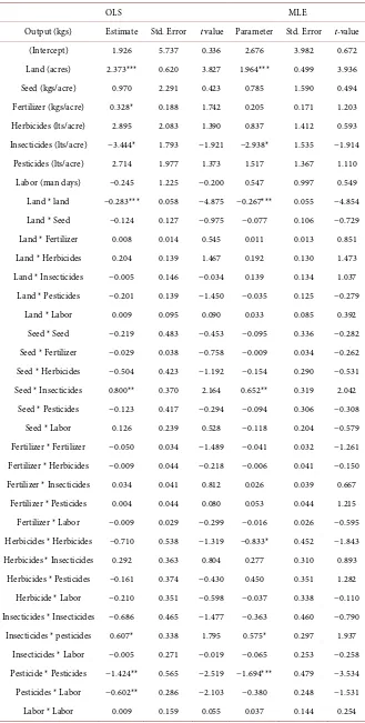
of the translog production function are presented in Table 1. The results show that 6 of the coefficients that represent first-order derivatives are significant and have the expected signs. Land size has the expected sign, and impacts the output level in kg/acre positively at the 1% significance level. Increasing the use of in-secticides decreases the level of outputwhich is unexpected; this is significant at the 10% level for both OLS and MLE models. This outcome perhaps could be explained by inappropriate use of insecticides [27].

The second-order derivatives for all inputs are negative, implying the con- cavity property holds for the existing farm technology. The _R2 is 95%. The _F

value is 147.9 and is significant at the 1% level. Lambda

( )

λ which measures the inefficiency variation in relation to the idiosyncratic variation computed as the ratio of standard errors of σu to σv has a value of 4.003 and is significant

at the 1% level. Gamma

( )

γ _{which is the ratio of the efficiency variation}

( )

2

u

σ

to the total variation

( )

σ

2 _{of parameters is 0.95. This implies that 95% of the} total output variation is due to production inefficiency while 5% is due to varia-tion from unobserved and measurement errors

( )

2

v

σ

.

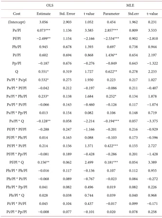
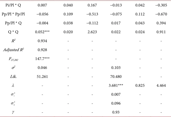
The translog cost frontier which is dual to the translog production frontier is shown in Table 2. It is econometrically estimated to provide the basis for com-puting both AE and EE. As mentioned earlier, the total cost and input prices were normalized by labor price per acre. The input prices included in the model are for seeds (Ps), fertilizer (Pf), herbicides (Ph), insecticides (Pi), and pesticides (Pp).

5.2. Efficiency Scores

TE, AE, and EE scores are reported in Table 3. The average TE score of the sampled wheat farms is 79%, with a minimum score of 37% and a maximum score of 97%. This implies that wheat farmers are not operating on the produc-tion frontier and can increase their TE score on average by as much as 21%. To achieve the TE score of the most efficient farmer, the output gain would be about 19% and 62% for the average farmer and the most inefficient farmer, re-spectively.

The average AE score is 80%, with a minimum score of 24% and a maximum score of 98%. This implies that on average allocative inefficiency (the lack of cost-minimizing behavior) accounts for a 20% loss in wheat income, or the po-tential to reduce cost (cost savings) by as much as 20%. To achieve the AE score of the most efficient farmer, the average farmer would realize a savings of about 18% of the total cost while the most inefficient farmer would reduce costs by as much as 76% of the total cost.

[image:13.595.209.538.87.738.2]

Table 1. Estimates for production function (OLS) and stochastic frontier (MLE).

OLS MLE

Output (kgs) Estimate Std. Error t value Parameter Std. Error t-value (Intercept) 1.926 5.737 0.336 2.676 3.982 0.672 Land (acres) 2.373*** 0.620 3.827 1.964*** 0.499 3.936 Seed (kgs/acre) 0.970 2.291 0.423 0.785 1.590 0.494 Fertilizer (kgs/acre) 0.328* 0.188 1.742 0.205 0.171 1.203 Herbicides (lts/acre) 2.895 2.083 1.390 0.837 1.412 0.593 Insecticides (lts/acre) −3.444* 1.793 −1.921 −2.938* 1.535 −1.914

Pesticides (lts/acre) 2.714 1.977 1.373 1.517 1.367 1.110 Labor (man days) −0.245 1.225 −0.200 0.547 0.997 0.549 Land * land −0.283*** 0.058 −4.875 −0.267*** 0.055 −4.854 Land * Seed −0.124 0.127 −0.975 −0.077 0.106 −0.729 Land * Fertilizer 0.008 0.014 0.545 0.011 0.013 0.851 Land * Herbicides 0.204 0.139 1.467 0.192 0.130 1.473 Land * Insecticides −0.005 0.146 −0.034 0.139 0.134 1.037 Land * Pesticides −0.201 0.139 −1.450 −0.035 0.125 −0.279

Land * Labor 0.009 0.095 0.090 0.033 0.085 0.392 Seed * Seed −0.219 0.483 −0.453 −0.095 0.336 −0.282 Seed * Fertilizer −0.029 0.038 −0.758 −0.009 0.034 −0.262 Seed * Herbicides −0.504 0.423 −1.192 −0.154 0.290 −0.531 Seed * Insecticides 0.800** 0.370 2.164 0.652** 0.319 2.042

Seed * Pesticides −0.123 0.417 −0.294 −0.094 0.306 −0.308 Seed * Labor 0.126 0.239 0.528 −0.118 0.204 −0.579 Fertilizer * Fertilizer −0.050 0.034 −1.489 −0.041 0.032 −1.261 Fertilizer * Herbicides −0.009 0.044 −0.218 −0.006 0.041 −0.150 Fertilizer * Insecticides 0.034 0.041 0.812 0.026 0.039 0.667

Fertilizer * Pesticides 0.004 0.044 0.080 0.053 0.044 1.215 Fertilizer * Labor −0.009 0.029 −0.299 −0.016 0.026 −0.595 Herbicides * Herbicides −0.710 0.538 −1.319 −0.833* 0.452 −1.843 Herbicides * Insecticides 0.292 0.363 0.804 0.277 0.310 0.893

Herbicides * Pesticides −0.161 0.374 −0.430 0.450 0.351 1.282 Herbicide * Labor −0.210 0.351 −0.598 −0.037 0.338 −0.110 Insecticides * Insecticides −0.686 0.465 −1.477 −0.363 0.460 −0.790 Insecticides * pesticides 0.607* 0.338 1.795 0.575* 0.297 1.937

Continued

R2 _{0.950 - - - - -}

Adjusted R2 _{0.943 - - - - -}

F35,274 147.9*** - - - - -

σ2 _{0.050 - - 0.114 - -}

Lik. 42.770 - - 57.698 - - λ - - - 4.003*** 0.881 4.542

2

v

σ - - - 0.007 - -

2

u

σ _{- - - 0.108 - -}

2 2

u

σ γ

σ

= - - - 0.95 - -

[image:14.595.205.539.288.737.2]

***, **, and * represent the significance level at 1%, 5%, and 10%, respectively.

Table 2. OLS and MLE estimates of translog cost function.

OLS MLE

Cost Estimate Std. Error t value Parameter Std.err t-value (Intercept) 3.056 2.903 1.052 0.454 1.962 0.231

Ps/Pl 4.073*** 1.136 3.585 2.857*** 0.809 3.533 Pf/Pl −2.499** 1.154 −2.166 −2.534*** 0.902 −2.810 Ph/Pl 0.945 0.678 1.393 0.697 0.738 0.944

Pi/Pl 0.602 0.694 0.868 1.436** 0.654 2.197 Pp/Pl −0.187 0.676 −0.276 −0.849 0.643 −1.322

Q 0.551* 0.319 1.727 0.622** 0.278 2.233 Ps/Pl * Ps/pl 0.532* 0.275 1.930 0.223 0.217 1.027 Ps/Pl * Pf/Pl −0.042 0.212 −0.197 −0.086 0.211 −0.407 Ps/Pl * Ph/Pl 0.233* 0.138 1.684 0.252* 0.134 1.878

Ps/Pl * Pi/Pl −0.066 0.143 −0.460 −0.126 0.117 −1.074 Ps/Pl * Pp/Pl 0.013 0.154 0.082 0.106 0.148 0.719

Ps/Pl * Q −0.128** 0.058 −2.214 −0.194*** 0.057 −3.375 Pf/Pl * Pf/Pl −0.288 0.247 −1.166 −0.201 0.216 −0.929 Pf/Pl * Ph/Pl 0.014 0.163 0.088 −0.103 0.173 −0.596 Pf/Pl * Pi/Pl 0.214 0.156 1.371 0.422*** 0.155 2.727 Pf/Pl * Pp/Pl −0.081 0.189 −0.428 −0.286 0.201 −1.428

Pf/Pl * Q 0.156** 0.062 2.499 0.181*** 0.054 3.389 Ph/Pl * Ph/Pl −0.016 0.117 −0.136 0.107 0.112 0.955 Ph/Pl * Pi/Pl −0.068 0.089 −0.767 −0.023 0.084 −0.272 Ph/Pl * Pp/Pl 0.041 0.082 0.496 0.019 0.082 0.226

Continued

Pi/Pl * Q 0.007 0.040 0.167 −0.013 0.042 −0.305 Pp/Pl * Pp/Pl −0.056 0.109 −0.513 −0.075 0.112 −0.670 Pp/Pl * Q −0.004 0.038 −0.112 0.017 0.043 0.394

Q * Q 0.052*** 0.020 2.623 0.022 0.024 0.911

R2 _{0.934 - - - - -}

Adjusted R2 _{0.928 - - - - -}

F27,282 147.7*** - - - - -

σ2 _{0.046 - - 0.103 - -}

Lik. 51.261 - - 70.480 - -

λ - - - 3.681*** 0.825 4.464

2

v

σ - - - 0.007 - -

2

u

σ _{- - - 0.096 - -}

γ _{- - - 0.93 - -}

[image:15.595.214.538.86.309.2]

***, **, and * represent the significance level at 1%, 5%, and 10%, respectively.

Table 3. TE, AE, and EE for wheat production (pooled sample).

Min Max Mean Std.

TE 0.37 0.97 0.79 0.133

AE 0.24 0.98 0.80 0.125

EE 0.09 0.93 0.64 0.178

least efficient farmer could increase output and reduce cost by 90%.

5.3. Distribution of Efficiency Scores

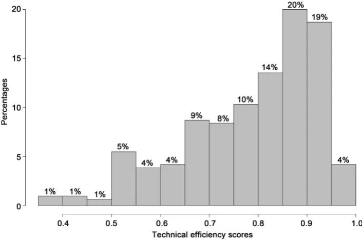
Figure 3 shows that the distribution of TE scores for the pooled survey sample is negatively skewed. The mean TE score for the pooled sample is ~80%, with 57% of the sampled farmers scoring above the average and 43% scoring below the av-erage (Table 3). Figure 4 shows that AE score is negative skewed. The mean AE score for the pooled sample is 80%, with 37% of the sampled farmers scoring below the average and 63% scoring above the average (Table 3). The minimum EE score is 64%, with 42% of the sampled wheat farmers operating below the average EE score. Figure 5 depicts the histogram of EE scores shows a negative skewness, implying that the median is on the right of the mean score.

5.4. Factors Influencing Efficiency

In contrast to input and output factors used in estimating efficiency scores, household idiosyncratic factors were analyzed to explore sources of inefficiencies for the pooled sample data of the study area. Also, each ward’s specific location was considered to capture heterogeneity in soil fertility, distance to urban areas, and infrastructure accessibility effect on TE, AE, and EE.

[image:15.595.208.538.352.421.2]

con-tract participation and farmers’ association memberships since they are the in-dicators of farmers’ participation in the value chain (coordination). Table 4

shows that with the ignorability condition (without considering sample selection bias), participation in contracts and farmers’ associations positively and signifi-cantly (5%, 1%, 1% level) influences TE, AE, and EE, respectively.

[image:16.595.185.538.203.438.2]

Conversely, age has a negative and significant (at the 5% level) effect on TE, AE, and EE. This suggests that older farmers are less efficient than younger far-

Figure 3. The distribution of TE scores of the pooled sample in the study area.

[image:16.595.185.538.480.716.2]

[image:17.595.188.538.79.326.2]

Figure 5. The distribution of EE scores of the pooled sample in the study area.

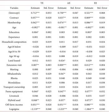
Table 4. Factors influencing efficiency (Tobit model).

TE AE EE

Variales Estimate Std. Error Estimate Std. Error Estimate Std. Error (Intercept) 0.712*** 0.053 0.730*** 0.047 0.521*** 0.068

[image:17.595.187.539.374.735.2]

mers. This result is plausible given that younger farmers are more receptive of new technologies and agricultural practices that increase production and mi-nimize costs. This finding is consistent with those of other studies that found the managerial capability to allocate factors of production in cost-minimizing beha-vior decreases with age [28]. The coefficient of education is positively and statis-tically significant at the 10% level for TE and EE. This result indicates that the higher the level of education, the higher the TE and EE. Farmers with more education are more likely to adopt better farm management practices that im-prove their levels of efficiency. As to be expected, extension services (visits) in-fluence TE, AE, and EE positively and significantly at the 5%, 1%, and 1% level, respectively. On-farm training conducted by extension officers enables farmers to acquire better and more cost-effective farm management practices. Off-farm income influences TE, AE, and EE positively and significantly at the 1% level. This could be because off-farm income facilitates purchases of factors of produc-tion at a certain point in time. A similar result is found in Chavas et al. [29]. Farm equipment is essential for wheat production in the study area, with own-ership influencing TE, AE, and EE positively at the 10%, 5%, and 5% significance levels, respectively. Ownership of modern farm equipment ensures carrying out various operations in a timely mannerand at a lower cost compared to hired ser-vices. Hybrid seeds which are known to yield higher production output in wheat crops have a positive and significant (5%, 10%, and 5% level) impact on TE, AE, and EE, respectively. The per unit cost of hybrid seed becomes lower than that of local seed because the production level of local seed is lower.

Land rent positively influences AE at the 10% significance level by maximiz-ing profit while minimizmaximiz-ing cost. Thus, farmers select best farm management practices that minimize their production costs to realize higher profits at pre-vailing market prices. In addition, the Mbulumbulu ward farmers seem to be better at minimizing costs than their counterparts in the other three surveyed wards that have better infrastructures and market accessibility. Mbulumbulu was the only surveyed ward where its farmers significantly operate with a least-cost combination at the 10% significance level.

5.5. Impact of Value Chain Participation on Efficiency

As mentioned earlier, we examined the impact of value chain participation on TE, AE, and EE. PSM was used to ascertain the sample selection bias of obser-vables. Nearest neighbor and caliper radius matching algorithms were used to match the characteristics of both participants and nonparticipants. We found that the levels of efficiency rise when farmers participate in vertical and hori-zontal coordination.

5.5.1. Vertical Coordination Impact

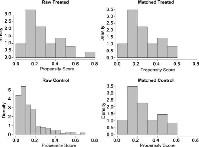
sample before and after matching. Because the distribution of participants (matched-treated) is dissimilar to the distribution of matched nonparticipants (matched-control), the TE effect of 6.2% under NN is still biased.

[image:19.595.208.540.170.416.2]

The matched participant and nonparticipant distributions under a caliper radius of 0.005 were similar (Figure 7). Out of 51 vertical coordination participants, 31 were dropped given a 0.005 caliper radius compared to only 2 being dropped

Figure 6. Vertical coordination histograms before and after matching by Nearest Neigh-bor algorithm of ratio 1:1.

[image:19.595.208.541.456.702.2]

given a 0.13 caliper radius (Table 5). Increasing the caliper radius to 0.13, we obtained suitable similar matches (Figure 8) for the matched-treated and matched- controlled observations. An attempt to further increase the radius to accommo-date at least 1 more participant did not prove worthwhile because the distribu-tions between matched participants and nonparticipants became dissimilar.

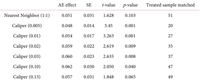
[image:20.595.210.540.277.520.2]

The results show that participation in vertical coordination as measured by contracts with buyers increases TE by 6.8% more for participants than for non-participants. This finding is significant at the 5% level (Table 5). Likewise, ver-tical coordination participation under the caliper radius of 0.13 improves AE by 5.7% more than its counterpart at the 10% significance level (Table 6). As in both the TE and AE cases, vertical coordination participation under a caliper ra-dius of 0.13 improves EE by 8.7% more for participants than for nonparticipants at the 5% significance level (Table 7).

Figure 8. Vertical coordination histograms before and after matching by caliper radius of 0.13.

Table 5. TE effect due to participation in vertical coordination.

TE effect SE t-value p-value Treated sample matched Nearest Neighbor (1:1) 0.062 0.031 2.011 0.044 51

[image:20.595.207.540.581.730.2]

[image:21.595.208.540.90.226.2]

Table 6. AE effect due to participation in vertical coordination.

AE effect SE t-value p-value Treated sample matched Nearest Neighbor (1:1) 0.051 0.031 1.628 0.103 51

[image:21.595.208.539.257.393.2]

Caliper (0.005) 0.048 0.014 3.45 0.001 20 Caliper (0.01) 0.054 0.017 3.263 0.001 27 Caliper (0.02) 0.059 0.022 2.619 0.009 35 Caliper (0.03) 0.060 0.023 2.635 0.008 37 Caliper (0.10) 0.062 0.030 2.050 0.040 47 Caliper (0.13) 0.057 0.031 1.848 0.065 49

Table 7. EE effect due to participation in vertical coordination.

TE effect SE t-value p-value Treated sample matched Nearest Neighbor (1:1) 0.077 0.043 1.779 0.075 51

Caliper (0.005) 0.061 0.021 2.940 0.003 20 Caliper (0.01) 0.075 0.026 2.901 0.004 27 Caliper (0.02) 0.091 0.032 2.892 0.004 35 Caliper (0.03) 0.097 0.032 2.984 0.003 37 Caliper (0.10) 0.095 0.0414 2.298 0.022 47 Caliper (0.13) 0.087 0.043 2.031 0.042 49

Table 8. TE effect due to participation in horizontal coordination.

TE effect SE t-value p-value Treated sample matched Nearest (1:1) 0.077 0.021 3.785 0.000 122

Caliper (0.03) 0.061 0.017 3.544 0.000 109 Caliper (0.04) 0.064 0.018 3.585 0.000 113 Caliper (0.05) 0.063 0.018 3.534 0.000 114

5.5.2. Horizontal Coordination Impact

As in the case of vertical coordination, an attempt was made to use the nearest neighbor (NN) technique for horizontal coordination matching. The results are shown in Table 8 for farmers who participated in horizontal coordination as measured by farmers’ association memberships. The results indicate an im-provement in TE of 7.7% for participants compared to non-participants. How-ever, the results are biased because the histogram distributions for matched- treated and matched-control groups are dissimilar (Figure 9). Thus, the need for a better matching procedure for the sample is important.

[image:21.595.207.540.424.513.2]

the matched distributions for treated and control groups were dissimilar like in the nearest neighbor (NN) matching procedure in Figure 9. Therefore, with a caliper radius of 0.05, horizontal coordination participants were found to im-prove their TE by 6.3% more than nonparticipants at the 1% significance level. Using a caliper radius of 0.05 for matched participants and nonparticipants, hori-zontal coordination as measured by farmers’ association memberships improved AE by 9.5% more for participants than for nonparticipants at the 1% significance level (Figure 10). There was no significant difference in the AE effect across the matching methods, implying good observations for the matches (Table 9). Likewise, with a caliper radius of 0.05, participants improved their EE by 11.6% more than did nonparticipants at the 1% significance level (Table 10).

6. Conclusions and Recommendations

The general objective of this study was to explain why wheat production is not responding to the increasing demand for wheat products in Tanzania. One fac-tor considered to explain the situation was the efficiency levels of wheat produc-tion units. TE, AE, and EE were first estimated over the pooled sample without the consideration of selection bias for participants and nonparticipants of the value chain. We employed the translog functional form for production and cost functions in a stochastic frontier analysis. Land, fertilizer, and insecticides were found to significantly influence the level of wheat output. The translog cost function revealed that seed, fertilizer, and insecticide prices monotonically in-creased with production cost, except for fertilizer price which violated the mo-notonicity assumption at the 5% significance level. Total production cost was found to significantly increasewith the quantity of wheat output, which means

[image:22.595.208.541.457.703.2]

[image:23.595.207.540.64.313.2] [image:23.595.206.540.376.460.2]

Figure 10. Horizontal coordination histograms before and after matching by caliper ra-dius of 0.05.

Table 9. AE effect due to participation in horizontal coordination.

AE effect SE t-value p-value Treated sample matched Nearest (1:1) 0.101 0.018 5.688 0.000 122

Caliper (0.03) 0.096 0.016 5.927 0.000 109 Caliper (0.04) 0.096 0.0167 5.769 0.000 113 Caliper (0.05) 0.095 0.017 5.722 0.000 114

Table 10. EE effect due to participation in horizontal coordination.

EE effect SE t-value p-value Treated sample matched Nearest (1:1) 0.132 0.026 5.080 0.000 122

Caliper (0.03) 0.115 0.023 5.076 0.000 109 Caliper (0.04) 0.117 0.023 5.019 0.000 113 Caliper (0.05) 0.116 0.023 4.959 0.000 114

that the monotonicity assumption of translogcost function holds for existing production technology.

The mean TE, AE and EE scores are all less than 100% implying that using the same factors of production at existing market prices, wheat farmers can signifi-cantly increase their output if appropriate policies or programs are implemented to improve the efficiency of wheat production. EE could be increased by 36% when TE and AE are attained. The factors that influenced TE, AE, and EE the most were contracts, farmers’ association memberships, education, extension visits, farm equipment, hybrid seed, and off-farm income.

[image:23.595.207.539.492.573.2]

the PSM technique reduces biases associated with observed variables. Using ca-liper radius matching, the vertical and horizontal coordination participants

im-prove their TE, AE, and EE scores more than do nonparticipants. Further

comparisons show that vertical cordination participation improves TE more than horizontal coordination participation. Also horizontal coordination par-ticipation improves AE more than vertical coordination parpar-ticipation. The im-plication is that vertical coordination is about honoring the contractual agree-ment put forth by buyers on various aspects including the technical require-ments and quantity to be deliverd. Accordingly, the farmers tend to utilize their factors of production more efficiently when meeting their contractual obliga-tions, resulting in a greater level of technical efficiency compared to allocative efficiency. _{On the other hand, horizontal coordination is about working in}

groups where most transactions are done in bulk thus reducing the cost of pro-duction per unit. Buying inputs and selling output jointly is advantageous to farmers because it is a cost-mimizing strategy. Thus, farmers who join associa-tions produce more at the least-cost combination which has a more direct im-plication on allocative efficiency than on technical efficiency.

Overall, our results recommend that in order to improve farm-unit efficiency, farmers need to participate in the value chain (vertical and horizontal coordina-tion) as it has been proven that participation improves farm-level efficiency. In addition, modern farm technology, higher education, and extension services empower farmers to increase their farm-level output and efficiency. Lastly, more off-farm employment activities are needed to supplement on-farm income to purchase more factors of production.

The scope of this paper was on application of SFA and PSM approaches to analyze efficiency using firsthand data collected from Northern part of Tanzania. The future direction should focus on using panel data if available with large sample size across the country where more representatives will be included in the analysis. This is because the regional heterogeneity of weather condition for wheat production across the country could bring varied efficiency levels that might call for a different policy measures. Also it would be fruitful to analyze in details factors that motivates and barriers that prevent wheat producers from value chain participation.

References

[1] Boselie, D., Henson, S. and Weatherspoon, D. (2003) Supermarket Procurement Practices in Developing Countries: Redefining the Roles of the Public and Private Sectors. American Journal Agricultural Economic Association, 85, 1155-1161.

https://doi.org/10.1111/j.0092-5853.2003.00522.x

[2] Neven, D. and Reardon, T. (2004) The Rise of Kenyan Supermarkets and the Evolu-tion of Their Horticulture Product Procurement Systems. Development Policy Re-view, 22, 669-699. https://doi.org/10.1111/j.1467-7679.2004.00271.x

[3] Hernandez, R., Reardon, T. and Berdegue, J. (2007) Supermarkets, Wholesalers, and Tomato Growers in Guatemala. Agricultural Economics, 36, 281-290.

[4] Minten, B., Randrianarison, L. and Swinnen, J. (2007) Spillovers from High-Value Agriculture for Exports on Land Use in Developing Countries: Evidence from Ma-dagascar. Agricultural Economics,37, 265-275.

https://doi.org/10.1111/j.1574-0862.2007.00273.x

[5] Neven, D., Odera, M., Reardon, T. and Wang, H. (2009) Kenyan Supermarkets, Emerging Middle-Class Horticultural Farmers, and Employment Impacts on the Rural Poor. World Development, 37, 1802-1811.

[6] Mason, N., Jayne, T. and Shiferaw, B. (2012) Wheat Consumption in Sub-Saharan Africa: Trends, Drivers, and Policy Implication.

http://fsg.afre.msu.edu/papers/idwp127.pdf

[7] Mburu, S., Ackello-ogutu, C. and Mulwa, R. (2014) Analysis of Economic Efficiency and Farm Size : A Case Study of Wheat Farmers in Nakuru District, Kenya. Eco-nomics Research International, 2014, Article ID: 802706.

https://doi.org/10.1155/2014/802706

[8] Temu, A. (2006) Aid for Trade and Agro-Based Private Sector Development in Tanzania. http://www.oecd.org/trade/aft/37563905.pdf

[9] Greene, W. (2010) A Stochastic Frontier Model with Correction for Sample Selec-tion. Journal of Productivity Analysis, 34, 15-24.

https://doi.org/10.1007/s11123-009-0159-1

[10] Jondrow, J., Knox Lovell, C., Materov, I. and Schmidt, P. (1982) On the Estimation of Technical Inefficiency in the Stochastic Frontier Production Function Model. Journal of Econometrics, 19, 233-238.

[11] Pitt, M. and Lee, L. (1981) The Measurement and Sources of Technical Efficiency in the Indonesian Weaving Industry. Journal of Development Economics, 9, 43-64. [12] Bogetoft, P. and Otto, L. (2015) Benchmark and Frontier Analysis Using DEA and

SFA. https://cran.r-project.org/web/packages/Benchmarking/Benchmarking.pdf [13] Bogetoft, P. and Otto, L. (2011) Benchmarking with DEA, SFA, and R. Springer-

Verlag, New York.

[14] Bravo-Ureta, B. and Rieger, L. (1991) Dairy Farm Efficiency Measurement Using Stochastic Frontiers and Neoclassical Duality. American Journal of Agricultural Economics, 73, 421-428. https://doi.org/10.2307/1242726

[15] Henningsen, A. (2010) Estimating Censored Regression Models in R Using the CensReg Package. R Package Vignettes Collection, 5, 12.

[16] Henningsen, A. (2015) Censored Regression (Tobit) Models.

https://cran.r-project.org/web/packages/censReg/censReg.pdf

[17] Mayen, C., Balagtas, J. and Alexander, C. (2010) Technology Adoption and Tech-nical Efficiency: Organic and Conventional Dairy Farms in the United States. Ame- rican Journal of Agricultural Economics, 92, 181-195.

https://doi.org/10.1093/ajae/aap018

[18] Caliendo, M. and Kopeinig, S. (2008) Some Practical Guidance for the Implementa-tion of Propensity Score Matching. Journal of Economic Surveys, 22, 31-72.

https://doi.org/10.1111/j.1467-6419.2007.00527.x

[19] Smith, J. and Todd, P. (2005) Does Matching Overcome Lalonde’s Critique of Nonexperimental Estimators? Journal of Econometrics, 125, 305-353.

[20] Rosenbaum, P. (2002) Observational Studies. 2nd Edition, Springer, New York. [21] Bravo-Ureta, B., Greene, W. and Solis, D. (2012) Technical Efficiency Analysis

Correcting for Biases from Observed and Unobserved Variables: An Application to a Natural Resource Management Project. Empirical Economics, 43, 55-72.

[22] Abate, G., Francesconi, G. and Getnet, K. (2014) Impact of Agricultural Coopera-tives on Smallholders’ Technical Efficiency: Empirical Evidence from Ethiopia. An-nals of Public and Cooperative Economics, 85, 257-286.

https://doi.org/10.1111/apce.12035

[23] Dehejia, R. and Wahba, S. (2002) Propensity Score-Matching Methods for Nonex-perimental Causal Studies. Review Economics and Statistics, 84, 151-161.

https://doi.org/10.1162/003465302317331982

[24] Christensen, L., Jorgenson, D. and Lau, L. (1973) Transcendental Logarithmic Pro-duction Frontiers. The Review of Economics and Statistics, 55, 28-45.

https://doi.org/10.2307/1927992

[25] Coelli, T.J. (1996) A Guide to DEAP Version 2.1: A Data Envelopment Analysis (Computer) Program. CEPA Working Paper 96/08, University of New England, Armidale.

[26] Food and Agriculture Organization (2013) Analysis of Incentives and Disincentives for Wheat in the United Republic of Tanzania. FAO, Rome.

[27] Chen, R., Huang, J. and Qiao, F. (2013) Farmers’ Knowledge on Pest Management and Pesticide Use in Bt Cotton Production in China. China Economic Review, 27, 15-24.

[28] Coelli, T., Rahman, S. and Thirtle, C. (2002) Technical, Allocative, Cost, and Scale Efficiencies in Bangladesh Rice Cultivation: A Non-Parametic Approach. Journal of Agricultural Economics, 53, 607-626.

https://doi.org/10.1111/j.1477-9552.2002.tb00040.x

[29] Chavas, J.-P., Oetruem, R. and Roh, M. (2005) Farm Household Production Effi-ciency: Evidence from the Gambia. American Journal of Agricultural Economics, 87, 160-179. https://doi.org/10.1111/j.0002-9092.2005.00709.x

Submit or recommend next manuscript to SCIRP and we will provide best service for you:

Accepting pre-submission inquiries through Email, Facebook, LinkedIn, Twitter, etc. A wide selection of journals (inclusive of 9 subjects, more than 200 journals)

Providing 24-hour high-quality service User-friendly online submission system Fair and swift peer-review system

Efficient typesetting and proofreading procedure

Display of the result of downloads and visits, as well as the number of cited articles Maximum dissemination of your research work