Munich Personal RePEc Archive
Least squares estimation for GARCH
(1,1) model with heavy tailed errors
Preminger, Arie and Storti, Giuseppe
Ben Gurion University of the Negev, Beer-Sheva, Israel., University
of Salerno, Italy
17 January 2014
Online at
https://mpra.ub.uni-muenchen.de/59082/
Least squares estimation for GARCH (1,1)
model with heavy tailed errors
∗
Arie Preminger
†Giuseppe Storti
‡October 4, 2014
Abstract
GARCH (1,1) models are widely used for modelling processes with time varying volatility. These include financial time series, which can be particularly heavy tailed. In this paper, we propose a log-transform-based least squares estimator (LSE) for the GARCH (1,1) model. The asymptotic properties of the LSE are studied under very mild moment conditions for the errors. We establish the consistency, asymptotic normality at the standard convergence rate of √n for our estimator. The finite sample properties are assessed by means of an extensive simulation study. Our results show that LSE is more accu-rate than the quasi-maximum likelihood estimator (QMLE) for heavy tailed errors. Finally, we provide some empirical evidence on two fi-nancial time series considering daily and high frequency returns. The results of the empirical analysis suggest that in some settings, depend-ing on the specific measure of volatility adopted, the LSE can allow for more accurate predictions of volatility than the usual Gaussian QMLE.
JEL Classification: C13, C15, C22.
Keywords: GARCH (1,1), least squares estimation, consistency, asymp-totic normality.
∗The authors thank Christian M. Hafner, for helpful comments. Giuseppe Storti grate-fully acknowledges funding from the Italian Ministry of Education, University and Re-search (MIUR) through PRIN project ”Forecasting economic and financial time series: understanding the complexity and modelling structural change” (code 2010J3LZEN).
†Ben Gurion University of the Negev, Beer-Sheva, Israel. E-mail: [email protected]
1
Introduction
In the last three decades there has been a large amount of theoretical and em-pirical research on modelling the conditional volatility of financial time series data. These time series, which appear to be uncorrelated, exhibit dependence in their squares, a notable example being the daily financial returns. The practical motivation lies in the increasing need to explain and to model risk and uncertainty usually associated with financial returns. One of the most successful approaches for modelling volatility makes use of the generalized autoregressive conditionally heteroskedasticity (GARCH) model, suggested by Bollerslev (1986), and its numerous extensions. Indeed, its simplicity and intuitive appeal make the GARCH model, especially the GARCH(1,1), a good starting point in many financial applications, see e.g. Hansen and Lunde (2005).
The main approach for the estimation of GARCH models is the quasi-maximum likelihood estimator (QMLE) approach where the estimates are obtained through maximization of a Gaussian likelihood function. Bollerslev and Wooldridge (1992) derived the asymptotic distribution of the QMLE under high level assumptions. When the errors have finite fourth moment the consistency and asymptotic normality of the QMLE for the GARCH(1,1) have been established by Lee and Hansen (1994) and Lumsdaine (1996). These results were extended to the case of GARCH (p,q) by Boussama (1998), Berkes et al. (2003) and Francq and Zako¨ıan (2009). However, empirical evidence indicates that for many financial time series, the distribution of errors is far from being Gaussian and it is usually heavy tailed (Hall and Yao (2003), Mittnik and Rachev (2000). Hall and Yao (2003) studied the QMLE for heavy tailed errors (without finite fourth moment). They showed that the asymptotic distribution may be non-Gaussian and the convergence rate is slower than√n. Straumann (2005) established similar results for a more general class of GARCH type models.
following cases: i) in the presence of heavy tailed or skewed error distributions ii) when the volatility persistence is close to unity. It is important to note that both these features typically occur in the analysis of financial time series. The paper also presents an empirical application to financial data whose aim is to evaluate the ability of the LSE to adequately reproduce the volatility dynamics of some commonly encountered classes of asset returns. To cover a wide range of features typically arising in financial applications, we con-sider two different datasets characterized by substantially different volatility patterns namely the daily log-returns on the S&P 500 stock market index and the 30 minutes log-returns on the US dollar/Swiss franc (USD/CHF) exchange rate. The results indicate that the LSE can produce more accurate predictions of volatility than the usual GQMLE. Further, in order to inves-tigate if the LSE is able to adequately characterize the stochastic structure of the two datasets analyzed, we compare the theoretical autocorrelation functions of squared returns implied by the estimated volatility models to their sample counterparts. In both cases the results are compared with those yielded by the GQMLE.
The structure of the paper is as follows. In Section 2 we discuss the LSE and derive its asymptotic properties. In Section 3 we conduct a simulation study aiming at investigating the small sample properties of the estimator, while the results of an application of the proposed estimation approach to two financial time series are presented in Section 4. Section 5 concludes. The mathematical proofs are presented in the Appendix.
We use the following notations throughout the paper. |A|= (tr(A′A))1/2
denotes the Euclidian norm of a vector or a matrix and ||A||r = (E(|A|r))1/r
denotes the Lr-norm of a random vector or matrix. The symbol →
D denotes
converges in distribution. The symbol →
a.s. (→p ) denotes convergence almost
surely (in probability). oa.s.(1) denotes a series of random variables that
converges to zero almost surely (a.s.).
2
Least squares estimation for the GARCH
(1,1) model
The standard GARCH (1,1) model as proposed by Bollerslev (1986) is given by
yt=
p
where {εt} is a sequence of independent and identically distributed (iid)
random variables with E(εt) = 0 and
h0t=ω0+α0yt2−1+β0h0t−1 (2)
The process is described by an unknown parameter vector θ0 = (ω0, α0, β0)′.
If E(ε2
t) = 1 then h0t is the conditional variance of yt given the history of
the system. However, without any moment conditions,h0.5
0t is the conditional
scaling parameter of the observed process. Let c0 = E[ln(ε2t)] and assume
that c0 is finite, which is implied by our assumptions below. By squaring the
terms in (1) and taking the logarithm we obtain
zt = ln(h0t) +ηt (3)
wherezt= ln(y2t)−c0andηt= ln(ε2t)−c0 are zero mean iid random variables.
This nonlinear regression can be estimated via a least squares estimation. Conditional on some initial positive value ˜h1(e.g. ˜h1 = ω), the objective
function is given by
˜
Qn(θ) = 21nPtn=1ℓ˜t(θ) = 21nPnt=1(zt−ln ˜ht(θ))2 (4)
where θ = (ω, α, β)′ and ˜h
t(θ) is defined recursively, fort≥2 by
˜
ht(θ) =ω+αyt2−1+β˜ht−1 (5)
The LSE of θ is defined as any measurable ˆθn of
ˆ
θn= arg min θ∈Θ
˜
Qn(θ) (6)
where Θ⊂(0,∞)×[0,∞]2. It will also be convenient to work withh
t(θ) the
unobserved conditional variance
ht(θ) = ω+αyt2−1+βht−1(θ) (7)
whereh1 is initialised from its stationary distribution. Note thath0t=ht(θ0)
and ˜h0t = ˜ht(θ0). For the unobserved process we construct the following
unobserved objective function
Qn(θ) = 21nPnt=1(zt−lnht(θ))2 = 21nPnt=1ℓt(θ) (8)
The primary difference between the two objective functions is that Qn(θ) is
choice of the initial values does not matter for the asymptotic properties of the LSE.
To show the strong consistency, the following assumptions will be made.
Assumptions
(A1) Θ ≡ {θ : 0 < ω ≤ ω ≤ ω,¯ 0 ≤ α ≤ α ≤ α,¯ 0 ≤ β ≤ β ≤ β <¯ 1}, where θ0 ∈Θ.
(A2) γ =Eln(α0ε2t +β0)<0
(A3)E|εt|2s <∞ for some s >0.
(A4) limr→0r−(1+δ)Pr(ε2t ≤r)<∞ for some δ >0.
Remark 1: The first assumption allows for the possibility that the process is a pure ARCH or even an iid. process. Nelson (1990) showed that As-sumption A2 is sufficient and necessary for strict stationarity of (1) and (2).
Note that by Jensen’s inequality Assumption A2 holds if α0 +β0 ≤ 1 and
E(ε2
t) = 1. But the condition does not require that α0+β0 ≤ 1. Thus, we
are allowing for the possibility of mildly explosive GARCH, in addition to
integrated GARCH. However, this conclusion does not necessarily hold if εt
has infinite second moment. Nelson (1990) shows that when εt is standard
Cauchy, γ = 2Eln(β0.5
0 +α00.5), so that the set of parameter values which
allows for strict stationarity is smaller than the set α0+β0 <1. Assumption
A3 is a mild moment condition which allows for heavy tailed errors. Assump-tion A4 implies that the distribuAssump-tion of the error term is not concentrated around zero, and one sufficient condition is that the density ofεt is bounded.
This condition is necessary for both consistency and asymptotic normality. A similar condition also appears in Berkes et al.(2003). Assumptions A3 and A4 imply that zt, ηt are finite a.s. and the scaling factor c0 is finite (see
Lemma 1(iii) in the Appendix for details).
Theorem 1: Under Assumptions A1-A4, θˆn → a.s.θ0
The next theorems establish the asymptotic normality for our estimator. For
GQMLE the former result is obtained under the assumption that E(ε4
t)<∞.
For the LSE, we consider the additional assumption:
(A5) θ0 ∈Θ0, where Θ0 denote the interior of Θ.
Remark 3: Assumption A5 is needed to establish the asymptotic normality, otherwise when the parameters are on the boundary other methods should
be used. For example, under the null hypothesis that α= 0, the conditional
volatility process is degenerate which implies that β is unidentifiable and
the null value of α is on the boundary, so its distribution cannot be normal. Andrews (2001) and Francq and Zakoian (2007) study in detail the distri-bution of the QMLE in that case. This issue is beyond the scope of this paper.
We can now derive the LSE asymptotic distribution.
Theorem 2: Under Assumptions A1-A5, √n(ˆθn−θ0)→
D N(0,Ω), where
Ω = κJ−1, J = E (J
t), Jt= h12 0t
∂h0t ∂θ
∂h0t
∂θ′ and κ= E(η
2
t).
Remark 4: Let ˆJt and ˆη2t be the sample counterparts of Jt and ηt2 where ˆθn
is used and the variance is conditional on some initial fixed value. Under Lemma 7, it is straightforward to show that ˆΩn= 1nPnt=1ηˆt2Jˆt, is a strongly
consistent estimate of Ω. Further, for the QMLE, it was shown that the covariance matrix estimate converges in probability to the true quantity (see e.g. Francq and Zakoian (2009)). It is worth nothing that the methods used in the Appendix can easily be applied to prove almost sure convergence to the true asymptotic covariance matrix also in the context of quasi-likelihood estimation.
Remark 5: An important use of the asymptotic normality shown in Theorem 2 is to construct a Wald statistic to test the null hypothesis,
H0 :Rθ0 =r
where R is a given k ×3 matrix and r is a given k ×1 vector. This test
statistic may be defined as
Wn=
Rθˆn−r
′
RΩˆnR′
−1
Rθˆn−r
and we reject H0 for large values of Wn. The following theorem gives the
limiting distribution of Wn under the null hypothesis.
Theorem 3: Under Assumptions A1-A5, Wn →
D χ
2
k,
Remark 6: Other scale measures can be used as our objective function. Thus,
instead of using the LSE one may use the Lq estimator in which the scale
measure is based on the q−th absolute moment (q≥1) of the fitted
residu-als. For example, for q = 1 the least absolute deviations estimator (LADE)
was proposed by Peng and Yao (2003). They showed that the LADE is
lo-cally asymptotilo-cally Gaussian with convergence rate √n provided that the
second moment of the error term is finite (see also Huang et al. (2008)). Another more general class of scale measures is the “regular scale about the origin”, introduced by Sakata and White (2001), which allows for more ro-bust estimation. The choice of a specific scale measure could be motivated by efficiency or robustness considerations. Further, the unique features of each estimation method should be considered before deriving its asymptotic properties for the GARCH case.
Remark 7: Our estimator can be treated as an alternative to the common GQMLE in cases where the error distribution does not have finite fourth mo-ment. For example, we can consider the Cauchy distribution or the Student
t distribution with≤4 degrees of freedom.
Remark 8: When the fourth order moment is assumed to be finite, the
GQMLE is √n consistent for the true parameter values. However, in the
presence of extreme non-normality, this estimator can fail to produce asymp-totically efficient estimates. Hence, a two-step estimation procedure can be applied to gain efficiency. In the first step the GQMLE is used to obtain a consistent estimate of the scaling parameter and in the second step the LSE is used to estimate the model parameters. The issue of efficiency will be examined in the simulation study in the next section.
Remark 9: In our setting, we assume that the scaling factor c0 is known.
This assumption is standard1. It simplifies the discussion and implies that
the practitioner has some a-priori knowledge or can formulate some reason-able assumptions about the distribution of the errors. Further, our empirical
1
results, shown in the next section, clearly indicate that our findings are not sensitive to the choice of the scaling factor.
Remark 10: If we treat c0 as unknown, (α0, ω0) can be estimated2 up to
a scale parameter. However, other GARCH estimation methods considered in the literature, R-estimation (Andrews (2012), M-estimation (Mukherjee (2008)), LAD-estimation (Peng and Yao (2003)), are also not used to di-rectly estimate θ0 = (ω0, α0, β0)′. Instead, those methods are used to
esti-mate (ω0/d, α0/d, β0)′ where d >0 is unknown when the error distribution
is unknown. Another approach is to assume that ω0 is known, see Linton el
al. (2010).
Remark 11: Estimating θ0 when c0 is unknown is more complicated and
requires modifying our estimation procedure. In what follows we describe in general, a possible estimation procedure for this case. However, investigating the asymptotic and empirical properties of the proposed estimator is left for future work. Note that from (1)-(2) and letting ¯h0t = h0t/ω0 = 1 +
(α0/ω0)y2t−1+β0¯h0t−1, we have
ln(yt2) =c0+ ln(¯h0t) +ζt (9)
where c0 = E[ln(ω0ε2t)] and {ζt} is a sequence of mean zero iid variables.
As mentioned above, this nonlinear regression can be estimated via a least squares estimation. Thus, the unknown parametersψ0 = (c0, α0/ω0, β0) are
estimated by minimizing the following modified objective function
˜
Qn(ψ) = 21nPnt=1(ln(y2t)−c−ln ˜¯ht(θ))2 (10)
where ψ = (c, θ′)′, θ = (α/ω, β)′ and ¯h
t(θ) = 1 + (α/ω)yt2−1+β¯ht−1(θ). In
order to fully identify θ0, we can use a standard two-step estimation
proce-dure, see e.g. White (1994). In the first step, we apply the modified LSE to obtain a consistent estimate for the normalized series {yt
¯
h00.t5}which should resemble √ω0εt for large samples. In the second step, given the identified
rescaled error distribution, θ0 can be identified3 via the maximum likelihood
method (Rekkasa and Wong (2008); Francq and Zakoian (2013)).
2
Theβ parameter is invariant to rescaling of the error term.
3
A simple way to identify the parameters would be to assume that E(ε2
t) = 1, which implies
3
Simulation evidence
In this section, we investigate the finite sample properties of the LSE by means of a simulation study and compare the performance of the LSE with that of the GQMLE for a wide range of processes.
We note that for ˜θn, the GQMLE, √n(˜θn −θ0) ∼ N(0, κNJ−1) where
κN = E(ε4t)−1. This relationship implies that the variability of the LSE
relative to the GQMLE is captured by the efficiency ratio λ = κN/κ. The
larger this quantity is, the more efficient the LSE is relative to the GQMLE. This relative efficiency depends on the distribution of the error term. The efficiency ratio for error distributions that have been used in the simulation study and have finite fourth moment are shown in Table 1. The results imply that the LSE can be substantially more efficient than the GQMLE when the distribution of the error term deviates from normality.
Table 1: : Efficiency of the LSE relative to GQMLE for different error dis-tributions.
Distributions κ κN λ
Normal 4.92 2 0.41
t5 6.47 19.12 2.96
χ2
1−1 4.67 64.55 13.81
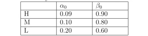
In the simulation study, in order to reflect a wide range of situations commonly encountered in practical financial modelling, we have considered different levels of persistence for the volatility model as well as different dis-tributions for the errors. In particular, three different volatility parameteri-zations are used corresponding to three different levels of persistence in the volatility model: High (H), Medium (L) and Low (L). The selected volatility models have been summarized in Table 2. For each model in the table, the value of ω0 in the volatility model was determined in order to constrain the
[image:10.595.165.424.619.683.2]variance of each of the DGP to be equal to 1.
Table 2: : Volatility models used for the simulation study.
α0 β0
H 0.09 0.90
M 0.10 0.80
L 0.20 0.60
Student’s t, with 3 and 5 degrees of freedom, and standardized χ2
1. It is
worth noting that E(ε4
t) < ∞ for all the distributions except for the t3. In
this case the asymptotic normality of the GQMLE is not expected to hold (Straumann (2005), p. 178).
Then, considering four different sample sizes,T = 500,1000,2000,5000, a set of 1000 pseudo-random time series was simulated from each of the DGP’s obtained matching the assumed error distributions with the volatil-ity models summarized in Table 2. Next, a GARCH(1,1) model was fitted to each of the simulated series by using the GQMLE and the LSE,
respec-tively. In particular, two different versions of the LSE have been used 4.
First, assuming knowledge of the underlying error distribution, the LSE was implemented using the correct scaling factor c0. This can be easily
approxi-mated by simulating a very large sample5 from the assumed distribution for
error term. Then, ˜c0, a simulated approximation of c0 can be obtained by
taking the sample average of the natural logarithms of the squared simulated values. Furthermore, we also considered a two-stage LSE. In the first stage the GQMLE is used to obtain ˆc0, a consistent estimate of the scaling
fac-tor. In the second stage the model is re-estimated by our method using the estimated scaling factor.
In order to assess the quality of the estimates, we have focused on the simulated values of bias and Mean Square Error (MSE). For the sake of brevity and ease of exposition, the results obtained for the two stage LSE have been omitted since they did not turn out to be significantly different from those obtained for the estimator based on the correct scaling factor (˜c0). Also, to simplify the presentation of the results, we omit reporting the
bias and MSE values for the constant term ω0. However this set of results is
available from the authors upon request.
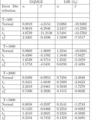
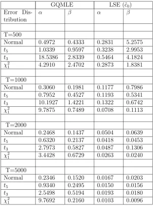
A different situation appears for the High persistence GARCH model. In this case the GQMLE, differently from the LSE, is characterized by non-regular behaviour. Even in the case of normal errors, for large sample sizes, the value of the MSE is surprisingly higher than that registered for the LSE. This is probably due to the fact that the chosen DGP is very close to the border of the weak stationarity region. In the case of t5 errors the LSE is
by far more efficient than the QMLE if a sufficiently large sample size is
considered (T ≥2000). In the remaining cases the LSE is performing better
than the QMLE, in terms of MSE, for all the sample sizes considered.
4
The GQMLE was computed by using the MATLAB function fminunc to maximize the associated quasi likelihood function with respect to the unknown parameters. For the LSE, the relevant sum of squares was minimized using the MATLAB function lsqnonlin.
5
It is interesting to note that, in general, the bias tends to be positive for the ARCH coefficientαwhile it is always negative for the GARCH coefficient
β. This result is not surprising since it is in line with previous findings in the literature (see e.g. Straumann, 20056). Furthermore, we must note that the
overall behaviour observed in the cases of Low and Medium volatility per-sistence (see tables 3-6) is substantially different from that registered for the High persistence case (see tables 7-8). For the Low and Medium persistence models, in line with the results in Table 1, the GQMLE is performing sub-stantially better than the LSE in the Gaussian case while, in non-Gaussian settings, the overall performance of the LSE model tends to improve over its competitor.
4
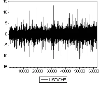
An application to financial data
In this section we present the results of an application of the proposed es-timator to two time series of financial returns. First, we consider a time series of daily (percentage) log-returns on the S&P 500 index from January 5, 1971 to May 30, 2006 for a total of 8937 observations (Figure 1). Second, we consider a time series of 30 minutes returns on the USD/CHF exchange rate from April 1, 1996 to March 30, 2001 for a total of 62495 observations (Figure 2). In the latter case the data have been standardized in order to account for the presence of some observations exactly equal to zero. In order to remove any serial correlation structure, the S&P 500 series has been pre-filtered fitting an AR(2) model to the raw returns. Differently, the USD/CHF intraday exchange rate returns series has been pre-filtered in two steps: i) an AR(1) model has been fitted to the standardized returns to account for serial correlation ii) we have corrected for intraday seasonal patterns in volatility dividing the filtered returns by the corresponding seasonal factors. These have been calculated by simply averaging the squared returns in the various intraday intervals and taking square roots.
The performance of the LSE in reproducing the volatility of returns has been compared with that of the classical GQMLE. To evaluate the sensitivity of the LSE to different choices of the scaling factor, we consider estimatingc0
under different distributional assumptions for the error series: a standardized
t5, a standard normal and a Cauchy random variable with location and scale
parameters equal to 0 and 1, respectively. In order to assess the relative performance of the estimators considered, we use the squared returns as a
6
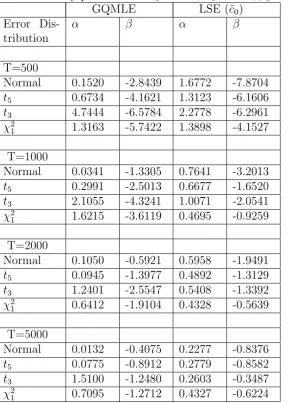
Table 3: : Simulated bias (x 100) over 1000 pseudo-random replicates for the Low persistence volatility process with ω0 = 0.20, α0 = 0.20, β0 = 0.60.
GQMLE LSE (˜c0)
Error Dis-tribution
α β α β
T=500
Normal 0.1520 -2.8439 1.6772 -7.8704
t5 0.6734 -4.1621 1.3123 -6.1606
t3 4.7444 -6.5784 2.2778 -6.2961
χ2
1 1.3163 -5.7422 1.3898 -4.1527
T=1000
Normal 0.0341 -1.3305 0.7641 -3.2013
t5 0.2991 -2.5013 0.6677 -1.6520
t3 2.1055 -4.3241 1.0071 -2.0541
χ2
1 1.6215 -3.6119 0.4695 -0.9259
T=2000
Normal 0.1050 -0.5921 0.5958 -1.9491
t5 0.0945 -1.3977 0.4892 -1.3129
t3 1.2401 -2.5547 0.5408 -1.3392
χ2
1 0.6412 -1.9104 0.4328 -0.5639
T=5000
Normal 0.0132 -0.4075 0.2277 -0.8376
t5 0.0775 -0.8912 0.2779 -0.8582
t3 1.5100 -1.2480 0.2603 -0.3487
χ2
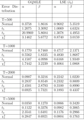
Table 4: : Simulated Mean Square Error (x 100) over 1000 pseudo-random replicates for the Low persistence volatility process withω0 = 0.20,α0 = 0.20,
β0 = 0.60.
GQMLE LSE (˜c0)
Error Dis-tribution
α β α β
T=500
Normal 0.3758 1.8616 0.9682 5.3519
t5 1.2075 3.3092 1.0069 4.6324
t3 20.9969 5.8684 1.3078 4.4953
χ2
1 3.1462 5.6772 0.8740 3.0159
T=1000
Normal 0.1770 0.7460 0.4717 2.1371
t5 0.5562 1.8335 0.4830 1.8687
t3 4.1587 4.0998 0.6168 1.9349
χ2
1 1.7442 3.2239 0.4064 1.0868
T=2000
Normal 0.0907 0.3216 0.2242 1.0220
t5 0.2837 0.8548 0.2332 0.8009
t3 2.4501 2.8793 0.3100 0.8990
χ2
1 0.6925 1.7321 0.1893 0.4337
T=5000
Normal 0.0350 0.1270 0.0866 0.3420
t5 0.1122 0.3376 0.0982 0.3065
t3 2.3541 1.6481 0.1176 0.2966
χ2
Table 5: : Simulated bias (x 100) over 1000 pseudo-random replicates for the Medium persistence volatility process with ω0 = 0.10,α0 = 0.10, β0 = 0.80.
GQMLE LSE (˜c0)
Error Dis-tribution
α β α β
T=500
Normal 0.0819 -4.3154 2.0268 -18.9382
t5 0.9619 -6.2946 2.2417 -14.2595
t3 4.0729 -11.2138 2.5491 -13.5762
χ2
1 2.4365 -9.4596 1.5899 -7.5517
T=1000
Normal 0.0669 -1.8689 1.2244 -10.0284
t5 0.4380 -3.1592 1.1640 -7.0427
t3 1.6529 -6.5714 1.2531 -5.2478
χ2
1 1.1753 -4.5431 0.6193 -2.4494
T=2000
Normal 0.0489 -0.9953 0.7294 -3.3948
t5 0.3451 -1.6849 0.5889 -2.0423
t3 2.2618 -2.9461 0.5049 -1.7278
χ2
1 0.7206 -2.3926 0.1515 -0.6626
T=5000
Normal 0.0058 -0.3597 0.3141 -1.2743
t5 0.1450 -0.6466 0.2254 -0.8282
t3 1.4510 -2.0021 0.2324 -0.5920
χ2
Table 6: : Simulated Mean Square Error (x 100) over 1000 pseudo-random replicates for the Medium persistence volatility process with ω0 = 0.10,α0 =
0.10, β0 = 0.80.
GQMLE LSE (˜c0)
Error Dis-tribution
α β α β
T=500
Normal 0.2022 1.8818 0.5225 11.4787
t5 0.5860 2.8612 0.5130 7.9819
t3 7.4474 5.5943 0.7750 7.9700
χ2
1 1.9106 4.8282 0.3737 4.1705
T=1000
Normal 0.0814 0.6311 0.2662 5.4332
t5 0.3151 1.3267 0.2441 3.6226
t3 1.8726 2.9159 0.2570 2.5763
χ2
1 0.5817 2.1179 0.1246 1.0478
T=2000
Normal 0.0393 0.2548 0.1130 1.3540
t5 0.1139 0.5641 0.1061 0.8534
t3 2.6353 1.6702 0.1128 0.6794
χ2
1 0.2732 0.9862 0.0564 0.2240
T=5000
Normal 0.0163 0.0831 0.0419 0.2913
t5 0.0477 0.1737 0.0353 0.1521
t3 1.0281 0.9039 0.0410 0.1307
χ2
Table 7: : Simulated bias (x 100) over 1000 pseudo-random replicates for the High persistence volatility process with ω0 = 0.01,α0 = 0.09, β0 = 0.90.
GQMLE LSE (˜c0)
Error Dis-tribution
α β α β
T=500
Normal 0.9561 -2.3596 1.1684 -8.7027
t5 2.6349 -4.3835 1.5388 -5.8657
t3 5.9734 -7.9647 2.0560 -7.3836
χ2
1 5.1557 -7.4965 1.3561 -3.6250
T=1000
Normal 1.3435 -1.8156 0.5509 -2.1848
t5 2.4439 -2.7361 0.6940 -1.7094
t3 4.4315 -4.8574 0.6724 -1.8669
χ2
1 5.3084 -3.6914 0.4448 -0.7459
T=2000
Normal 1.4091 -1.3727 0.2109 -0.5496
t5 2.0595 -1.6655 0.1693 -0.4252
t3 3.1710 -3.0927 0.2558 -0.4894
χ2
1 3.7968 -2.6326 0.2052 -0.2945
T=5000
Normal 1.6350 -1.5051 0.1300 -0.2902
t5 1.9663 -1.2381 0.0633 -0.1555
t3 2.9075 -2.0648 0.1768 -0.2310
χ2
Table 8: : Simulated Mean Square Error (x 100) over 1000 pseudo-random replicates for the High persistence volatility process withω0 = 0.01,α0 = 0.09,
β0 = 0.90.
GQMLE LSE (˜c0)
Error Dis-tribution
α β α β
T=500
Normal 0.4972 0.4333 0.2831 5.2575
t5 1.0339 0.9597 0.3238 2.9953
t3 18.5386 2.8339 0.5464 4.1824
χ2
1 4.2910 2.4702 0.2873 1.8381
T=1000
Normal 0.3060 0.1981 0.1177 0.7986
t5 0.7952 0.4527 0.1193 0.5341
t3 10.1927 1.4221 0.1322 0.6742
χ2
1 9.7875 0.7489 0.0708 0.1113
T=2000
Normal 0.2468 0.1437 0.0504 0.0639
t5 0.6320 0.2137 0.0418 0.0453
t3 2.7973 0.5827 0.0487 0.1306
χ2
1 3.4428 0.6729 0.0263 0.0240
T=5000
Normal 0.2346 0.1520 0.0167 0.0203
t5 0.9340 0.2495 0.0150 0.0156
t3 2.5498 0.5194 0.0193 0.0180
χ2
proxy of volatility and then refer to the following well-known loss functions: the Mean Square Error (MSE), the QLIKE, the Mean Absolute Error (MAE) and its equivalent formulation in terms of standard deviations (MAE-SD). A discussion of these loss functions and their properties can be found in Patton (2011). For MSE and QLIKE, the expected loss is minimized if the volatility estimate used to compute the loss function coincides with the true conditional variance. Differently, for MAE and MAE-SD, optimality is achieved in correspondence of the true conditional median of the squared returns.
The volatility of each of the two series, S&P 500 and USD/CHF exchange rate returns, has been modelled as a GARCH(1,1) whose parameters have been estimated by QML and by the LSE (Table 9). For the S&P 500, the
estimates of the ARCH coefficient α obtained by the LSE are substantially
lower than that yielded by the GQMLE while the opposite applies to the
GARCH parameterβ. Furthermore, it is interesting to analyze the behaviour
of the different estimators under the four loss functions considered (Table 8). For the MSE, all the estimators yield very similar performances. The only exception is given by the LSE constructed under the assumption of Cauchy errors which is characterized by a value of the MSE much higher than was observed for its competitors.
A different picture arises if we consider the QLIKE criterion. For the daily S&P 500 returns series, except for the Cauchy case, the performance of LSE is quite close to that of the GQMLE. The gap substantially increases in the case of the 30 minutes USD/CHF exchange rate returns. For the other two loss functions considered, MAE and MAE-SD, and for both datasets, the LSE is always outperforming the QMLE. The LSE performance is optimized if we estimate the scaling constant c0 under the assumption of Cauchy errors
with location and scale parameters equal to 0 and 1, respectively. However, in general, it is worth noting that the performance of the LSE appears to be quite robust to the choice of the scaling factor c0.
The message we get from these results is that, if one is interested in the conditional variance of returns as a measure of volatility, no clear advantage derives from using the LSE instead of the usual GQMLE. Differently, if the focus is on an alternative measure of volatility, such as the conditional median of squared returns, the use of the LSE can potentially allow for substantial accuracy gains.
Table 9: GARCH(1,1) parameter estimates under different estimators (* x 10−4). Key to table: LS-D is the Least Squares estimator under distribution
D (N=Normal, C=Cauchy, t5= Student’s with 5 df.)
S&P 500 USD/CHF
ω α β ω α β
QML 0.0007* 0.0658 0.9271 0.0448 0.0832 0.8752
LS-N 0.0036 0.0395 0.9486 0.0615* 0.1293 0.8302
LS-t5 0.0030 0.0322 0.9478 0.0499* 0.1030 0.8312
[image:22.595.105.491.540.646.2]LS-C 0.0013 0.0131 0.9386 0.0208* 0.0374 0.8259
Table 10: Evaluation of volatility estimates for the daily S&P 500 and 30 min. USD/CHF returns by means of different loss functions: MAE, MSE and MSE-LOG. Key to table: LS-D is the Least Squares estimator under
distribution D (N=Normal, C=Cauchy, t5= Student’s with 5 df.)
S&P 500 USD/CHF
MSE QLIKE MAE
MAE-SD
MSE QLIKE MAE
MAE-SD
QML 34.63 0.72 1.06 0.53 14.69 0.90 1.19 0.60
LS-N 34.53 0.74 0.99 0.49 14.77 1.45 1.08 0.53
LS-t5 34.56 0.82 0.93 0.46 14.76 1.73 1.02 0.50
of Cauchy errors since in this case the autocorrelation function of squared returns cannot be defined. Also, for the USD/CHF exchange rate returns series, the set of model coefficients estimated using LSE violate the condition for the existence of a finite fourth moment which is
(3α2+ 2αβ +β2)<1
For this reason, it has been necessary to approximate the corresponding autocorrelation function by means of the formula proposed by Ding and Granger (1996) for conditionally Gaussian GARCH(1,1) models
ρ(k) = (α+β)k−1
α+ β 3
, k≥1
where ρ(k) is the lag k autocorrelation function of a squared GARCH(1,1)
process. For the daily S&P 500 returns series, it is evident how the LSE is interpolating the decay of the sample autocorrelation function of squared returns much better than the QML approach. Differently, for the 30 minutes USD/CHF exchange rate returns series, the autocorrelation patterns implied by the t5-LSE and QMLE result quite close while the normal LSE drastically
overestimates the value of the autocorrelation function of squared returns.
5
Conclusions and future work
In this paper, we suggest using LSE for the estimation of a GARCH (1,1) model. The estimator is based on the log transformation of the squared data. We establish the consistency and asymptotic normality of the proposed esti-mator. Our results have been obtained under mild regularity conditions that allow for heavy tailed error distributions that can be of particular interest in financial applications. Its finite sample properties have been investigated via a simulation study, which shows that, in the presence of extreme non-normality, the proposed LSE can allow for some efficiency gains with respect to the QMLE. We also provide empirical evidence that applying the LSE can yield better volatility forecasts than the standard QMLE. Our estimates also fit quite well the autocorrelation function of the squared returns.
When working with high frequency returns, an important issue is the ro-bustness of the estimation procedure, since these data are typically charac-terized by a high fraction of very small returns, which, after the log transfor-mation, can produce large negative values. Therefore, our estimator, which
is based on the L2 scale measure, may not be optimal in the presence of
Appendix
Throughout the Appendix,K will denote a generic positive number that may
vary in different uses. To simplify the notation we set
˙
hit(θ) =
∂ht(θ)
∂θi
, ¨hijt(θ) =
∂ht(θ)
∂θi∂θj
, h˙˜it(θ) =
∂˜ht(θ)
∂θi
, ¨˜hijt(θ) =
∂˜ht(θ)
∂θi∂θj
Let ∇ℓt(θ) = ∂ℓ∂θt(θ), ∇ℓit(θ) = ∂ℓ∂θt(iθ) and ∇2ℓt(θ) = ∂ℓ∂θ∂θt(θ)′, ∇
2ℓ
ijt(θ) = ∂θ∂ℓit∂θ(θ)j
denote the first and second derivatives of ℓt(θ) (and their elements),
respec-tively.
5.1
A. Proofs of theorems
Proof of Theorem 1:
We use similar arguments as in Theorem 5.3.1 of Straumann (2005, p.101) showing strong consistency by contradiction. Suppose that ˆθn6→θ0 a.s. so for
some arbitrary γ >0, the compact setF ={ω ∈Ω|lim supn→∞||θˆn−θ0|| ≥
γ, θˆn ∈Θ}has a positive probability. Since the set N = Θ∩ {θ :|θˆn−θ0| ≥
γ}is compact, there exists a non-null subset ¯F ⊂F such that for everyω ∈F¯, one can find inN, a convergent subsequenceˆθni(ω)→θ ∈N. By definition of
the LSE
lim inf
n→∞
1
ni
Pni
t=1ℓ˜t(θ0) ≥ lim infn
→∞ θinf∈N 1
ni
Pni t=1ℓ˜t(θ)
= lim inf
n→∞
1
ni
Pni
t=1ℓ˜t(ˆθni)
From Lemma 5,
lim inf
n→∞
1
ni
Pni
t=1ℓt(θ0) ≥ lim infn→∞ n1i
Pni
t=1ℓt(ˆθni) (11)
The inequality above and Lemmas 4(ii)-(iii) imply that with positive prob-ability Eℓt(θ0) ≥ E infθ∈Nℓt(θ). This result contradicts Lemma 4(i) which
states that in the limit Qn(θ) is uniquely minimized at θ0. Since γ > 0 is
arbitrary, the strong consistency follows.
Proof of Theorem 2: By Theorem 1, ¯θn → θ0 a.s. so for n sufficiently
mean-value expansion of ˜Qn(ˆθn) =Pnt=1ℓ˜t(ˆθn) around θ0, we have
0 = n−0.5Xn t=1∇
˜
ℓt(ˆθn) (12)
= n−0.5Xn
t=1∇
˜
ℓt(θ0) +
1
n
Pn
t=1∇2ℓ˜t(¯θn)
√
n(ˆθn−θ0)
= n−0.5Xn t=1∇
˜
ℓt(θ0)
+ h1nPn
t=1∇2ℓ˜t(¯θn)− 1
n
Pn
t=1∇2ℓt(¯θn)
+ 1nPn
t=1∇2ℓt(¯θn) +J
−Ji
√
n(ˆθn−θ0)
where ¯θn lies on the chord between ˆθn and θ0.
Lemma 6 and the asymptotic equivalence lemma (e.g. see White (1994), p.172) imply that √1nPnt=1∂ℓ˜t(θ0)
.
∂θ →
D N(0, H) where H =κJ and J is a
positive definite matrix. Next, Lemmas 7(i)-(ii) imply that the first and sec-ond terms, inside the square brackets in (12), converge a.s. to zero. Hence, to complete the proof it suffices to solve (12) and apply Slutsky’s theorem.
Proof of Theorem 3: The result follows immediately from Theorems 1-2 and Lemma 7.
B. Lemmata
Lemma 1: Under Assumptions A1-A4, for some p∈(0,1)
i) (y2
t, h0t) are strictly stationary and ergodic and E (hp0t)<∞, E (|yt|2p)<∞
ii)infθ∈Θℓt(θ), ℓt(θ), ∇ℓit(θ) and∇2ℓijt(θ) are strictly stationary and ergodic.
iii) E (η2
t)<∞
Proof:
i) Under Assumption A2, the result follows directly from (1)-(2) and Theo-rem 4 of Nelson (1990).
strictly stationary and ergodic (see Stout (1974), Theorem 3.5.8). The same result follows forℓt(θ) and its derivatives by Lemma 2(ii) of Lee and Hansen
(1994).
iii) Let w = ε2
t, F(x) = Pr(w ≤ x) and f(x) be the density function, since
ηt = w−c0, the result follows if
R+∞
0 [ln(w)]
2f(w)dw <∞. By integration
by parts
1
Z
0
[ln(w)]2f(w)dw= [ln(1)]2F(1)−
1
Z
r
ln(w)
w F(w)dw−
r
Z
0
ln(w)
w F(w)dw
The first integral on the RHS is bounded for any r >0. Hence, by Assump-tion A4, when r >0 is small enough, there exists some δ > 0 such that the second integral is bounded byKR r
0 w
δln(w)dw. This integral is finite for any
δ >0. Forw≥1 we getR+∞
1 [ln(w)]
2f(w)dw < R+∞
1 w
2sf(w)dw ≤ E|ε t|2s,
since ln(w)< ws/2 for any s >0, and the desired result follows by
Assump-tion A3.
Lemma 2: Under Assumptions A1-A4, for some p∈(0,1)
i) Esupθ∈Θ
ht(θ)−˜ht(θ)
p
=O( ¯βt) and E|sup
θ∈Θ˜ht(θ)|p < ∞.
ii) Esupθ∈Θ0
h˙it(θ)−h˙˜it(θ)
p
=O( ¯βt) for all i.
iii) Esupθ∈Θ0 ¨
hijt(θ)−¨˜hijt(θ)
p
=O( ¯βt) for all i, j.
Proof: i) By iterating (7) and using the fact α0yt2−1−i ≤ h0t, we get
ht(θ) = ω+αyt2−1+βht−1(θ) (13)
= Xt−1
i=0(ω+αy 2
t−1−i)βi+βth1(θ)
= X∞
i=0(ω+αy 2
t−1−i)βi
= ω
1−β +α
X∞
i=0β
iy2
t−1−i
≤ ω¯
1−β +
¯ α α0 X∞ i=0 ¯
Hence, the cr inequality ((a+b)q ≤ aq+bq for all a, b > 0, q ∈ [0,1]) and
Lemma 1(i) imply that for some p∈(0,1),
E|sup
θ∈Θ
ht(θ)|p ≤ K+KEhp0t < ∞ (14)
Now, without loss of generality, set ˜h1 = 0.5(¯ω +ω), by iterating (5) we
obtain
˜
ht(θ) =ω+αyt2−1+β˜ht−1(θ) =
Xt−1
i=0(ω+αy 2
t−1−i)βi+βt˜h1 (15)
Hence ˜
ht(θ)−ht(θ) = ω+αy2t−1+β˜ht−1(θ) =βt(˜h1−h1(θ)) (16)
and by (16),
E sup
θ∈Θ0
ht(θ)−˜ht(θ)
p
≤ βt(˜hp1+ E sup
θ∈Θ0|
h1(θ)|p)≤Kβ¯t (17)
Further, by Lemma 1(i) and the cr inequality
E(¯ω+ ¯αyt2−1−i)p <∞ (18)
and
E
sup
θ∈Θ
˜ht(θ)
p
≤Xti−=01E(¯ω+ ¯αyt2−1−i)pβ¯ip+ ¯βpth˜p1 <∞
ii) We start by showing that for some p∈(0,1) and all i,
E
sup
θ∈Θ0 ˙
hit(θ)
p
<∞ (19)
By (13) and the fact that y2
t−1−i ≤α0−1h0t,
∂ht(θ)
∂ω ≤
1
1−β (20)
∂ht(θ)
∂α =
X∞
i=0β
iy2
t−1−i ≤
1
α
hX∞
i=0αβ
iy2
t−1−i
i
≤ 1
αht(θ) (21)
∂ht(θ)
∂β =
X∞
i=1iβ
i(ω+αy2
t−1−i) (22)
≤ X∞i=1iβi
ω+ α
α0
h0t
≤ ω¯X∞
i=1i
¯
βi+ α¯
α0
X∞
i=0
¯
The term in (20) is bounded and admits moments of any order. As for (21)-(22), the result follows directly from the cr inequality and Lemma 1(i).
In view of (16), almost surely,
sup
θ∈Θ0
h˙it(θ)− ˙˜
hit(θ)
≤ tβ¯
(t−1)(˜h
1+ sup
θ∈Θ0
h1(θ)) + ¯βt sup
θ∈Θ0| ˙
hi1(θ)| ≤ Kβ¯t
the desired result follows by (14), (19) and the cr inequality.
iii) From (20)-(22) and direct calculations we get,
∂2h
t
∂ω2 =
∂2h
t
∂α2 =
∂2h
t
∂ω∂α = 0,
∂2h
t
∂ω∂β
1
β ≤
X∞
i=1i
¯
βi (23)
which are bounded and admit moments of any order. We also find
∂2h
t
∂α∂β ≤ α
X∞
i=1iβ
iy2
t−1−i ≤
¯
α α0
X∞
i=1iβ
ih
0t (24)
∂2h
t
∂β2 =
1
β
X∞
i=2i(i−1)(ω+αy 2
t−1−i)βi (25)
So, similar to Lemma 2(ii) we can show that for some 0 < p <1,
E
sup
θ∈Θ0 ¨hijt(θ)
p
<∞ (26)
for all i, j. In view of (16), almost surely,
sup
θ∈Θ0
¨hijt(θ)− ¨˜
hijt(θ)
≤ t(t−1) ¯β
(t−2)[˜h
1+ sup
θ∈Θ0
h1(θ)]
+ tβ¯(t−1) sup
θ∈Θ0| ˙
hj1(θ)|+ tβ¯t−1 sup
θ∈Θ0| ˙
hi1(θ)|
+ ¯βt sup
θ∈Θ0| ¨
hij1(θ)|
and by (14), (19), (26) and the cr inequality the desired result follows.
Lemma 37: Under Assumptions A1-A4, for all r≥1
7
i)
supθ∈Θ0h
−1
t (θ) ˙hit(θ)
r <∞ for all i
ii)
supθ∈Θ0h−
1
t (θ)¨hijt(θ)
r <∞ for all i, j
iii)
supθ∈Θ0 ˜
h−1
t (θ) ˙˜hit(θ)
r < ∞ for all i, and
supθ∈Θ0 ˜
h−1
t (θ)¨˜hijt(θ)
r < ∞
for all i, j.
Proof: i) Eq. (20) and (21) imply that the derivative of ht with respect
to ω and α (divided by ht) are bounded and hence admits moments of any
order. However, this is not true for the derivative with respect to β. From (13) we get ht(θ) ≥ ω+ (ω +αy2t−1−i)βi for all i ≥ 1. Using the fact that
x/(1 +x)< xp/r for allx≥0 and anyp∈(0,1),r≥1 (this idea of exploiting
this inequality is due to Boussama (2000)), we get
∂ht
∂β
1
ht ≤
1
β
X∞
i=1i
(ω+αy2
t−1−i)βi
ω+ (ω+αy2
t−1−i)βi
(27)
≤ β1X∞i=1i
(ω+αy2
t−1−i)βi
ω
p/r
≤ 1
βωp/r
X∞
i=1i
¯
βip/r(¯ω+ ¯αyt2−1−i)p/r
Therefore, by (18) and Minkowski’s inequality we get
sup
θ∈Θ0
∂ht ∂β 1 ht r
≤ KX∞
i=1i
¯
βi
E ¯ω+ ¯αyt2−1−ip1/r
<∞
ii) From (23)-(25), we observe that the relevant second derivatives satisfy
∂2h
t
∂β2
1
ht ≤
1
β
X∞
i=2i(i−1)
(ω+αy2
t−1−i)βi
ω+ (ω+αy2
t−1−i)βi
(28)
and
∂2h
t
∂α∂β ≤
X∞
i=1iβ
i (ω+αyt2−1−i)
ω+ (ω+αy2
t−1−i)βi
,
(the other derivatives are naturally bounded). Using the same arguments as in part (i) of the lemma the desired results follow.
Lemma 4: Under Assumptions A1-A5,
i) E(ℓt(θ0)) ≤ E(ℓt(θ)) with equality if and only if θ 6=θ0.
ii) For any compact set N⊆Θ,
lim inf
n→∞ θinf∈N 1
n
Pn
t=1ℓt(θ) ≥ E infθ∈Nℓt(θ).
iii) limn→∞ 1n
Pn
t=1ℓt(θ0) = Eℓt(θ0).
iv) E |supθ∈Θlnht(θ)|2<∞ and E(zt2)<∞
Proof:
i) Note that
E(ℓt(θ))−E(ℓt(θ0)) = 12E [(zt−lnht(θ))2−ηt2] (29)
= 12E [ln(h0t−ln(ht(θ))]2+ E [ln(h0t/ht)] E(ηt)
= 12E [ln (ht(θ0)/ht(θ))]2 ≥ 0
with equality if and only if ht(θ0) =ht(θ)a.s.
ii) For any compact set N⊆Θ we have,
lim inf
n→∞ θinf∈N 1
n n
P
t=1
ℓt(θ) ≥ lim infn→∞ n1 n
P
t=1
infθ∈Nℓt(θ) (30)
Further, note Eℓt(θ)<∞ is well defined and belongs to ℜ ∪ {+∞}. Hence,
by Lemma 1(ii), we can apply the ergodic theorem (see Billingsley (1995) p.284) to the stationary and ergodic sequence {infθ∈Nℓt(θ)}t to obtain
lim inf
n→∞ θinf∈N 1
n
Pn
t=1ℓt(θ) ≥ lim inf n→∞
1
n
Pn
t=1infθ∈Nℓt(θ) (31)
≥ E
inf
θ∈Nℓt(θ)
iii) Note that Eℓt(θ0) = E(η2t) < ∞ by Lemma 1(iii). The desired result
iv) Notice, that since 0< ω≤ht(θ) for any p >0,
ln(ω) ≤
sup
θ∈Θ
lnht(θ)
≤ K + sup
θ∈Θ
ht(θ)
p/2
By (14) we obtain that E |supθ∈Θlnht(θ)|2
< ∞. This result and Lemma 1(iii) also imply that E(z2
t) is finite.
Lemma 5: Under Assumptions A1-A4,
sup
θ∈Θ
1 n Pn t=1 ˜
ℓt(θ)−ℓt(θ)
a.s.→0
Proof:
Let At(θ) = ˜ℓt(θ)− ℓt(θ). To prove this result, it suffices to check that
E supθ∈Θ|At(θ)|q, is bounded by a summable sequence int, for some q ≥0.
Indeed then (by Markov inequality) for all λ >0,
X∞
t=1P(supθ∈Θ|At(θ)| > λ) ≤
X∞
t=1E supθ∈Θ|At(θ)|
q/λq <
∞ (32)
so that the Borel-Cantelli lemma implies that supθ∈Θ|At(θ)| converges to
zero a.s. This convergence and the Cesaro lemma imply the desired result. Now, since ˜ht, ht ≥ ω > 0, an application of the mean-value theorem
lead to
|ln ˜ht(θ)−lnht(θ)| ≤ K|˜ht(θ)−ht(θ)| (33)
So, from (4), (8) and the cr inequality, for some p∈(0,1)
E sup
θ∈Θ|
˜
ℓt(θ)−ℓt(θ)|p/4 ≤ E sup θ∈Θ
ln ˜ht(θ)−lnht(θ)
p/4
×
ln ˜ht(θ)−lnht(θ) + 2 (zt+ lnht(θ)) p/4 ≤ E " sup
θ∈Θ
˜ht(θ)−ht(θ) p/2
1 +zt+ sup θ∈Θ
lnht(θ)
p/4#
≤ KE
sup
θ∈Θ
˜ht(θ)−ht(θ)
p
=O β¯t
The second inequality holds by (33). The third inequality holds by the cr
by Lemma 2(i).
Lemma 6: Under Assumptions A1-A5,
i) n
−1/2Pn
t=1
∇ℓ˜t(θ0)− ∇ℓt(θ0)
→0 a.s.
ii)n−1/2Pn
t=1∇ℓt(θ0)→
D N(0, κJ) whereJ is positive definite andκ= E(η
2
t)
.
Proof:
i) We use the proof idea of Lemma 8 in Robinson and Zaffaroni (2006). Let.
Bt=∇ℓit(θ0)− ∇ℓ˜it(θ0), the gradients of (4) and (8) are given by
∇ℓ˜it(θ0) = (zt−ln ˜h0t)
˙˜
h0it
˜
h0t
, ∇ℓit(θ0) = (zt−lnh0t)
˙
h0it
h0t
=ηt
˙
h0it
h0t
(34)
where ˙h0it= ˙hit(θ0), h˙˜0it= ˙˜hijt(θ0). Hence,
Bt=∇ℓit(θ0)− ∇ℓ˜it(θ0) =ηt
˙
h0it
h0t −
˙˜
h0it
˜
h0t
!
+h˙˜˜0it
h0t
ln ˜h0t
h0t
!
and
n−1/2Xn
t=1Bt≤n
−1/2KXn
t=1ηt
˙
h0it−h˙˜0it
+ h˙˜0it
˜
h0t
h0it−˜h0it
(35)
Next, by application of the cr and Cauchy-Schwarz inequalities, we get that
P∞
t=1|Bt| has some finite p > 0 moment and thus by Loeve (p. 121) is a.s.
finite. Further Lemma 2(i)-(ii) implies that a.s. |Bt| ≤ Kβ¯t, ∀t. Hence, by
Kronecker lemma (35) tends to zero a.s. as n → ∞ and the desired result
follows
ii) From (34)
E (∇ℓit(θ0)|Ft−1) =
˙
h0it
h0t
E (ηt|Ft−1) =
˙
h0it
h0t
E (ηt) = 0
where Ft=σ(yt, yt−1, . . .) and
k∇ℓit(θ0)∇ℓjt(θ0)k ≤ E ηt2
˙
h0it
h0t
2 ˙
h0jt
h0t
by applying the Cauchy-Schwarz inequality and Lemmas 1(iii) and 3(i). Thus, we have shown that the second moment of each element of the gradient is finite hence E|∇ℓt(θ0)∇ℓt(θ0)′|<∞. These results and Lemma 1(ii) imply
that{∇ℓt(θ0),Ft}is a stationary, ergodic and martingale difference sequence
with finite variance
var(∇ℓt(θ0)) = E(ηt2)E
1
h2 0t
∂h0t
∂θ ∂h0t
∂θ′
=κJ
Next, by using similar arguments used in Lemma 5 in Lumsdaine (1996) we can show thatJ is a positive definite matrix. Thus, Theorem 23.1 of Billings-ley (1968) and the Cram´er-Wold device imply that n−1/2Pn
t=1∇2ℓt(θ0) →D
N(0, κJ).
Lemma 7: Under Assumptions A1-A5,
i) supθ∈Θ0 1 n Pn t=1
∇2ℓ˜
t(θ)− ∇2ℓt(θ)
→0 a.s.
ii) If ˜θn → a.s.θ0,
1
n
Pn
t=1∇2ℓt(˜θn)a.s.→ −J
Proof:
i) First, let Ct(θ) = ∇2ℓijt(θ) − ∇2ℓ˜ijt(θ). Using similar arguments as
in Lemma 5, it suffices to check that E supθ∈Θ0|Ct(θ)|q is bounded by a
summable sequence in t, for some q ≥ 0. Second, given (4) and (8) the
second derivatives are
∇2ℓ˜ijt(θ) = (zt−ln ˜ht)
¨˜
hijt
˜
ht
−(zt−ln ˜ht+ 1)
˙˜
hith˙˜jt
˜
h2
t
(36)
and
∇2ℓijt(θ) = (zt−lnht)
¨
hijt
ht −
(zt−lnht+ 1)
˙
hith˙jt
h2
t
(37)
Third, note
˙
hith˙˜jt
h2
t −
˙˜
hith˙˜jt
˜ h2 t ≤ K ( ˙ hit ht h ˙˜
hit−h˙it
i +h˙˜jt
˜
ht
h ˙˜
hjt−h˙jt
i )
Finally, using (36)-(38) we obtain
sup
θ∈Θ0
Ct(θ) ≤ sup θ∈Θ0
(
1 +ηt+ ln
h0t
ht
¨
hijt
ht −
¨˜
hijt
˜
ht
!
+˜h˜ijt
ht
ln ˜ht
ht
!
+ h˙ith˙jt
h2
t −
˙˜
hith˙˜jt
˜
h2
t
!
+ h˙˜ith˙˜jt ˜
h2
t
ln ˜ht
ht
!)
≤ K sup
θ∈Θ0
1 +ηt+ ln
h0t
ht
( ˜
hijt
ht
+ h˙˜it ˜ ht ˙˜ hjt ˜ ht !
ht−˜ht
+ h˙it
ht
˙˜
hit−h˙it
+h˙˜jt
˜
ht
˙˜
hjt−h˙jt
+¨hijt−¨˜hijt
)
By applying Holder and Minkowski inequalities with Lemmas 2, 3 and 4(iv), we get for some q ∈ (0,1) that E supθ∈Θ0|Ct(θ)|q = O( ¯βt) and the desired result follows.
ii) From (37), E (∇2ℓ
t(θ0)) = −J and
E sup
θ∈Θ0
∇2ℓijt(θ)
≤ E sup
θ∈Θ0
1 +ηt+ ln
h0t
ht
¨
hijt
ht
+ h˙ith˙jt
h2 t ! ≤
1 +||ηt||2+
sup
θ∈Θ0 ln
h0t
ht 2 ( sup
θ∈Θ0 ¨ hijt ht 2 + sup
θ∈Θ0 ˙ hit ht 4 sup
θ∈Θ0 ˙ hjt ht 4 ) <∞
The second inequality holds by applying the Cauchy-Schwarz and Minkowski inequalities. The last inequality holds by Lemma 1(iii), Lemmas 3 and 4(iv). From the ergodic theorem (see e.g., Billingsley (1995)),
sup
θ∈Θ0 1
n
Pn
t=1∇2ℓt(θ)−E (∇2ℓt(θ))
→
a.s.0
Hence, given ε >0
1 n Pn
t=1∇2ℓt(˜θn)−E
∇2ℓ
t(˜θn)
<
a.s. for n sufficiently large. Since E (∇2ℓ
t(θ)) is continues
E
∇2ℓijt(˜θn)
−E ∇2ℓijt(θ0)
<
1 2ε
a.s. for n sufficiently large since ˜θn →θ0 a.s. and the desired result follows
References
[1] Andrews B. (2012). Rank based estimation for GARCH processes.
Econo-metric Theory, 28(5), 1037-1064.
[2] Andrews D.W.K.(2001). Testing when a parameter is on the boundary of the maintained hypothesis.Econometrica, 69, 683-734.
[3] Berkes I. Horvath L. and P.S. Kokoszka (2003). GARCH processes:
struc-ture and estimation. Bernoulli, 9, 201-227.
[4] Berkes I. and L. Horvath (2003). The rate of consistency of the quasi-maximum likelihood estimator.Statistics and Probability Letters, 61, 133-143.
[5] Billingsley P. (1968) Convergence of Probability Measures. New York,
John Wiley.
[6] Billingsley P. (1995). Probability and Measure. New York, John Wiley.
[7] Bollerslev T. (1986). Generalized autoregressive conditional heteroskedas-ticity. Journal of Econometrics, 31, 307-327.
[8] Bollerslev T. and J.M. Wooldridge (1992). Quasi-maximum likelihood es-timation and inference in dynamic models with time-varying covariances.
Econometric Reviews, 11, 143-172.
[9] Boussama F. (2000). Normalit´e asymptotique de l’estimateur du
pesudo-maximum de vraisemblance d’un mode’le GARCH. C.R.Acad Sci.Paris,
331, 81-84.
[10] Dacorogna M.M., Gencay R., Muller U., Olsen R.B. and O.V. Pictet
(2001).An Introduction to High Frequency Finance. San Diego, CA:
Aca-demic Press.
[11] Ding, Z. and C. W. J. Granger (1996). Modelling volatility persistence
of speculative returns: a new approach, Journal of Econometrics, 73,
185–215.
[12] Francq C. and J-M. Zakoian (2007). Quasi-likelihood inference in
GARCH processes when some coefficients are equal to zero. Stochastic
[13] Francq C. and J-M. Zakoian (2009). A Tour in the asymptotic theory of
GARCH estimation,Handbook of Financial Time Series, 85-111, Berlin,
Springer-Verlag.
[14] Francq C. and J-M. Zakoian (2013). Estimating the marginal law of a time series with Applications to heavy-tailed distributions, Journal of Business and Economic Statistics, 31(4), 412-425.
[15] Hall P. and Q. Yao (2003). Inference in ARCH and GARCH models with heavy-tailed errors.Econometrica, 71, 285-317.
[16] Hansen P.R and A.Lunde (2005). A forecast comparison of volatility
models: does anything beat a GARCH(1,1)? Journal of Applied
Econo-metrics, 20(7), 873-889.
[17] Harvey A.C., Ruiz E. and N.G. Shephard (1994). Multivariate stochastic
variance models.Review of Economic Studies, 61, 247-264.
[18] Huang D., Wang H. and Q. Yao (2008). Estimating GARCH models:
when to use what? Econometrics Journal, 11, pp. 27–38
[19] Lee S.W. and B.E. Hansen (1994). Asymptotic theory for the
GARCH(1,1) quasi- maximum likelihood estimator. Econometric
The-ory, 10, 29-52.
[20] Linton O, Pan J. and H Wang (2010). Estimation for A non-stationary
semi-strong GARCH(1,1) models with heavy-tailed errors. Econometric
theory, 26(1), 1-28.
[21] Loeve M. (1977). Probability Theory 1, New York, Springer.
[22] Lumsdaine, R.L. (1996). Consistency and asymptotic normality of the quasi-maximum likelihood estimator in IGARCH(1,1) and covariance
sta-tionary GARCH (1,1) models. Econometrica, 64, 575-596.
[23] Mittnik S. and S.T. Rachev (2000) Stable Paretian Models in Finance.
New York, John-Wiley.
[24] Nelson D.B. (1990). Stationarity and persistence in the GARCH(1,1)
model. Econometric Theory, 6(3), 318-334.
[25] Mukherjee K. (2008). M-estimation in GARCH models. Econometric
[26] Patton A. (2011) Volatility forecast evaluation and comparison using imperfect volatility proxies.Journal of Econometrics, 160, 246–256.
[27] Peng, L. and Q. Yao (2003). Least absolute deviation estimation for
ARCH and GARCH models.Biometrika, 90, 967-975.
[28] Rekkasa M. and A. Wong (2008). Implementing likelihood-based infer-ence for fat-tailed distributions. Finance Research Letters, 5(1), 32-46.
[29] Robinson P.M. and P. Zaffaroni (2006). Pseudo-maximum likelihood es-timation of ARCH(∞) models. Annals of Statistics, 34, 1049–1074.
[30] Ruiz E. (1994). Quasi-maximum likelihood estimation of stochastic volatility models. Journal of Econometrics, 63, 289–306.
[31] Sakata S. and H. White (2001). S-estimation of nonlinear
regres-sion models with dependent and heterogeneous observations. Journal of
Econometrics, 103, 5-72.
[32] Stinchcombe M. B. and H. White (1992). Some measurability results
for extrema of random functions over random sets. Review of Economic
Studies, 59 (3), 495-514.
[33] Straumann D. (2005)Estimation in Conditionally Heteroscedastic Time
Series Models, Lecture Notes in Statistics, Springer.