A Web-based Tool to Evaluate the Iterative Processes of Direct Search Methods

A Web-based Tool to Evaluate the Iterative

Processes of Direct Search Methods

Pedro Mestre

Member, IAENG,

Aldina Correia

Member, IAENG,

Jo˜ao Matias

Member, IAENG,

Christophe Teixiera, Jos´e Almeida, Carlos Serodio

Member, IAENG

Abstract—Constrained and unconstrained Nonlinear Opti-mization Problems often appear in many engineering areas. In some of these cases it is not possible to use derivative based optimization methods because the objective function is not known or it is too complex or the objective function is non-smooth. In these cases derivative based methods cannot be used and Direct Search Methods might be the most suitable optimization methods. An Application Programming Interface (API) including some of these methods was implemented using Java Technology. This API can be accessed either by applications running in the same computer where it is installed or, it can be remotely accessed through a LAN or the Internet, using webservices. From the engineering point of view, the information needed from the API is the solution for the provided problem. On the other hand, from the optimization methods researchers’ point of view, not only the solution for the problem is needed. Also additional information about the iterative process is useful, such as: the number of iterations; the value of the solution at each iteration; the stopping criteria, etc. In this paper are presented the features added to the API to allow users to access to the iterative process data.

Index Terms—Nonlinear Optimization, Direct Search Me-thods, Java

I. INTRODUCTION

There are several areas of engineering where optimization problems must be solved. In some of these problems it is not possible to know which is its objective function, either because it is too complex or due to the costs involved in its determination (time, monetary, etc...). In other cases the derivatives of the objective function might be too complex to be determined or, the objective function might be non-smooth. In these cases it is not possible to use derivative-based optimization methods, as presented in [1]. In such problems one possible solution to cope with this is to use direct search methods that do not use derivatives or

Manuscript received March 05, 2011.

P. Mestre is with CITAB - Centre for the Research and Technology of Agro-Environment and Biological Sciences, University of Tr´as-os-Montes and Alto Douro, Vila Real, Portugal, email: [email protected]

A. Correia is with ESTGF-IPP, School of Technology and Management of Felgueiras Polytechnic Institute of Porto and CM-UTAD - Centre for the Mathematics, Portugal, [email protected]

J. Matias is with CM-UTAD - Centre for the Mathematics, Uni-versity of Tr´as-os-Montes and Alto Douro, Vila Real, Portugal, email: j [email protected]

C. Teixeira is with UTAD - University of Tr´as-os-Montes and Alto Douro, Vila Real, Portugal, email:cteixeira [email protected]

J. Almeida is with UTAD - University of Tr´as-os-Montes and Alto Douro, Vila Real, Portugal, email:[email protected]

C. Serˆodio is with CITAB - Centre for the Research and Technology of Agro-Environment and Biological Sciences, University of Tr´as-os-Montes and Alto Douro, Vila Real, Portugal, email: [email protected]

approximations to them. For further details see [2], [3] and [4].

Optimization problems that may appear can be of two natures: unconstrained optimization problems or constrained optimization problems. Unconstrained optimization problems have the form of (1):

min x∈Rn

f(x) ₍₁₎

where:

• f :_Rn→_Ris the objective function;

Constrained optimization problems have the form of (2):

min x∈Rn

f(x)

s.t. ci(x) = 0, i∈ E

ci(x)≤0, i∈ I

(2)

where:

• f :Rn→Ris the objective function;

• ci(x) = 0, i ∈ E, with E = {1,2, ..., t}, define the problem equality constraints;

• ci(x) ≤ 0, i ∈ I, with I = {t+ 1, t+ 2, ..., m}, represent the inequality constraints;

• Ω = {x∈Rn:ci= 0, i∈ E ∧ ci(x)≤0, i∈ I} is the set of all feasible points, i.e., the feasible region.

To solve both unconstrained and constrained optimization problems, an API (Application Programming Interface) was developed by the authors. The structure and functionalities of this API were presented in [5] and details on the methods that it implements and their performance analysis have been presented in [6], [7], [8], [9], [10] and [11].

It has been developed using Java Technology and sup-ports local and remote access [12]. This means that the methods implemented in the API can be accesses either by applications running in the same computer where the API is installed (local access), or it can be accessed remotely, through the Local Area Network (LAN) or the Internet, by applications running on remote computers (remote access). This remote access is made using webservices, allowing the API to be accessed by application developed in any programming technology.

the solution. So, some information about the iterative process of the several methods must be made available to the end user.

In this paper are presented the new features that were added to the developed API, which allow end users to access and visualise the iterative process data. Data is stored in a database and accessed trough a web server using a web browser. Both the database and the web server can be running in the same computer where the API is installed, for example when the API is installed in a server for remote access, or these services can be running in a remote computer.

Since in this paper the word ’method’ might have two different meanings, method to solve a problem or method in the context of Object Oriented Programming, in the first case the word will appear as ’method’ and in the second case as ’method’.

II. THEIMPLEMENTEDAPI

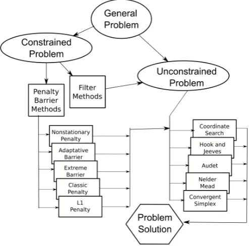
A detail of the the internal structure of the developed API is depicted in Fig. 1. When a problem is sent to the API, it can either be a constrained problem or an unconstrained problem. Depending on the type of problem several methods and algorithms are available. The methods currently implemented in the API do not use derivatives or approximations to them.

Figure 1. API Block Diagram

A. Solving unconstrained problems

The following five algorithms are available to solve un-constrained problems:

• A Coordinated Search algorithm, that can be analysed in detail in [1];

• Hooke and Jeves algorithm[4];

• An implementation of the algorithm of Audet et. al. as in [13], [14] and [15];

• The Nelder and Mead algorithm as in [16], or in [17] and [18];

• A Convergent Simplex algorithm can be analised in detail in analysed [1] and [19];

These algorithms are also used by the Internal Process of the methods implemented to solve constrained problems.

B. Solving constrained problems

Problems with constraints can be solved using one of the following two methods: Penalty and Barrier Methods; Filters Method.

1) Penalty and Barrier Methods: In Penalty and Barrier Methods the problem, in the form (2), is transformed into a sequence of problems in the form of (1), i.e., a sequence of unconstrained problems, which are then solved using the algorithms used to solve unconstrained problems. The new sequence of unconstrained problems that replaces problem

P is defined by:

Φ(xk, rk) : min xk∈Rn

f(xk) +rkp(x) (3)

whereΦis the new objective function,kis the iteration,pis a function that penalises (penalty) or refuses (barrier) points that violates the constraints and rk is a positive parameter.

The following five algorithms are available to solve un-constrained problems:

• A Nonstationary Penalty that can be analysed in [20]; • Adaptative Barrier as in [14], [15];

• Extreme Barrier as in [21] and [22]; • Classical Penalty as in [23], or in [24];

• `1Penalty which can be analysed in [25], [26] and [27];

2) Filters Method: The Filters Method, introduced by Fletcher and Leyffer in [28], unlike Penalty and Barrier Methods, consider optimality and feasibility separately. The constrained problems are considered as bi-objective pro-grams, and this method has as main goal the minimization of both the objective function (optimality) and a continuous function (h) that aggregates the constraint function values (feasibility).

Since it is not reasonable to have as a solution an infeasible point, priority must then be given toh. It must then be such that:

h(x)≥0 withh(x) = 0if and only ifxis feasible.

We can then define has:

h(x) =kC+(x)k, (4)

where k.k is the norm of a vector and C+(x)is the vector of the t+m values of the constraints in x, i.e, ci(x) for

i= 1,2, ..., t+m:

C+(x) =

ci(x) if ci(x)>0 0 if ci(x)≤0

C. Data to be stored

1) Input Data: Common to all methods, both the problem to be solved and the initial point at which the methods starts looking for the minimum must be stored.

The parameters needed by the Penalty and Barrier Method, and which are stored in the database are:

• The Penalty/Barrier function to be used;

• Initial parameters of the Penalty/Barrier function; • Minimum step length;

• Maximum value of the constraints violation; • Updating factor of the Penalty/Barrier function. For both the Penalty and Barrier Method and for the Filters Method, the parameters to be stored are:

• The maximum number of the external process iterations; • Tolerance distance between iterations;

• Tolerance between two values of the objective function (for two consecutive iterations);

• Method used in the internal process; • Parameters of the internal process.

In the filters method also the maximum initial value of for the constraints violations must be stored.

For the unconstrained methods, the data to be stored in the database are:

• Maximum number of iterations; • Initial step length;

• Tolerance for the distance between two iterations; • Tolerance between two values of the objective function

(for two consecutive iterations);

• Minimum step length.

These data for unconstrained methods are stored both when a unconstrained problem is solved, and when a con-strained problem is solved (parameters of the internal pro-cess).

2) Output Data: For all methods and algorithms, the solution to the problem xk and the value of the objective functionf(xk)are stored in the database.

The output values for the Penalty and Barrier Method stored in the database are:

• Number of external process iterations;

• Number of Penalty/Barrier function evaluations; • Value of the Penalty/Barrier function at the last iteration; • Penalty/Barrier function value at the best infeasible

solution;

• Iteration at which it was found the best infeasible solution;

• Constraint violation value at the best infeasible solution. The stored output parameters which are common to the Penalty and Barrier Method and the Filters Method are:

• Last iteration;

• Value of the objective function at the last iteration; • Best feasible solution if it exists;

• Value of the objective function at the best feasible solution;

• Iteration at which the best feasible solution was found; • Best infeasible solution if it exists;

• Value of the objective function at the best infeasible solution;

• Value of the constraints violation at the best infeasible solution.

For the Filters Method, also de following information is stored:

• Number of internal process iterations; • Number of objective function evaluations;

• Iteration where the best infeasible solution was found; • Set of non dominated solutions.

For the unconstrained methods, the output values stored in the database are:

• Number of objective function evaluations; • Last values calculated at the Stop Criteria; • The found solution;

• Value of the objective function at the found solution.

3) Iterative process Data: For each iteration (k) of the optimization method, it is stored in the database:

• The value k of the iteration; • The value of the approximation; • The value of the objective function;

III. DATA STORING ANDVISUALIZATION

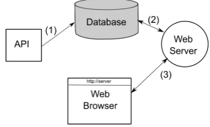
To allow the storage of the data from the execution of the methods, two new features must be added to the existing Java API: a database for data storage and a method to allow users to visualize and analyse the results. In the block diagram of Fig. 2 are presented the different blocks that make part of the proposed solution. It is composed by the existing API, a database server to store the data and a web server to supply the data to the user.

Figure 2. Block diagram of the proposed solution.

When an application invokes the run method of any optimization method of the API, prior to its execution, it sends to the database (1) the Input Data for that execution, as described in section II-C. After sending it the method starts its execution. While it is being executed, the API sends the Iterative Process Data to the database and when the execution finishes also all the Output Data are sent. The data from the execution is now ready to be accessed by the user.

All data is stored with an unique identifier associated to a particular execution. If a method is executed multiple times, data from all these executions will be stored in the database, each with an unique identifier. This identifier can be accessed by the application invoking the getIdentifier() me-thod.

to use a web browser that will contact the web server (3) and present information to the user as an World Wide Web page.

This architecture allows the different components to be all installed and running in the same computer, or, since all communications are made using TCP/IP (Transport Control Protocol / Internet Protocol), these components can be ins-talled in different computers. Two possible usage scenarios, among many, are:

• Local Access – The API, the database and the web server are all running in the same computer where the optimization methods are executed by the user, and it is the same computer where the user accesses to the data of the method execution. In this case, since all components are local, the user’s computer does not need to be connected to the network, but the user needs to install all components in his/her computer;

• Remote Access – The API is installed in the users’ computer and the database and the web server are installed in a remote server. In this case the user does not have to mind about the database server and web server installation, since he/she makes a remote access to the data. Data stored in the server can be shared with other users. However, to access the data the used computer must have a network access.

From the user’s point of view, this architectures allows the access to the data without the need for any kind of software installation. Independently of the location of the web server (local or remote) the user only needs to use a web browser and point it to the URL (Uniform Resource Locator) of the web server.

For the implementation of the database MySQL was chosen and the used web server is Apache Tomcat, which are freely available for installation. Therefore the pages in the server were developed using JSP (Java Server Pages).

A. Structure of the Database

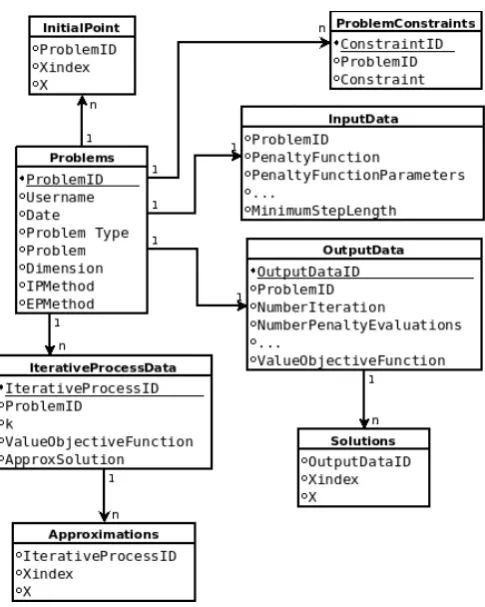
Based on the above presented requirements for data storage it was implemented the database presented in the ER-Diagram of Fig. 3.

In tableProblemsare stored a unique identifier for the problem (ProblemID), the name of the user (username) that requested the execution of the method, the date and the problem type (Unconstrained, Constrained or from the database of problems [12]). If the problem is not chosen from the database, it also stores the problem expression and dimension, and the expression of its constrains are stored in table ProblemConstrains. Also information about which methods were used in the External Process and the Internal Process are stored in this table (IPMethod and

EPMethod).

The parameters discussed in subsection II-C are stored in tables InputData, OutputData and

IterativeProcessData. Since the dimension of

the problem can vary form1ton, in tableSolutionsare stored the solutions to the problem. The number of entries in this table for each problem depend on the number of dimensions. The same is applicable to the tables that store the Initial Point and the Approximations to the solution.

Figure 3. ER Diagram of the database.

These three tables have a filed that contains the ID of the parent table, the solution (X1, X2, ...., Xn) in field X and its index (1,2, ...., n) in fieldXindex.

B. Modifications to the API code

For each optimization method implemented in the API it was needed to make some changes in their source code. The changes are related with addition of the methods to store the data, database configuration and enabling/disabling data logging into the database.

The list of new methods added to the implemented optimization methods is:

• void storeInDB(boolean flag) – used to

in-dicate the method if the data of the next execution is to be stored in the database or not. By default no information will be stored in the database;

• long getIdentifier()– returns the unique iden-tifier used in the database to store the data of the latest execution. Each call to therunmethodwill change this value (is data logging is enabled);

• void setDBHost(String hostname) – allows

to change the server on which the data will be stored. By default the API assumes that the MySQL server is installed in the same computer (localhost);

• void setDBUser(String username,

String password) – allows to set de username

and thepasswordfor the database server, if the default is not to be used;

• void setUsername(String username) –

page (see section III-C, Fig. 5). If no username is supplied, by default ”unknown” will be used.

The above presented methods are the public methods, added to the optimization methods, that make part of the API available to the programmer. Internally, other methods have been implemented to handle the establishment of the connection with the database and to send the data of the execution to it.

An example of code showing how to execute a method and store the data of the execution in the database is presented in Fig. 4. In the presented example the problem to be minimized is(x0−5)2+(x1−6)2, using(10.0,10.0)as the initial point and using the Coordinated Search algorithm to solve it. Be-cause the data of the execution is to be stored in the database, the method storeInDB() is called beforerun(). After the execution, the method getIdentifier()to get the identifier for that execution and it is presented in the console.

String expr = ‘‘(x0-5)ˆ2 + (x1-6)ˆ2’’; String initPoint = ‘‘x0=10.0 x1=10.0’’; CoordinatedSearch coord =

new CoordinatedSearch(expr,initPoit); coord.storeInDB(true);

coord.run();

long ID = coord.getIdentifier(); System.out.println("ID="+ID);

Figure 4. Java code to access the API, execute the Coordinated Search method and store the data in the default database.

C. Data Visualization

When the user accesses to the web server, he/she can choose from a list (Fig. 5) the problem to be visualized. The data that appears in the list of available problems are: the unique execution identifier, generated for each execution; the problem that was sent to the method to be solved; the user (if known) that requested the execution of the method; the execution date. The username parameter is always known if the user is using the remote access to the API feature (see [12]). Otherwise the setUsername() method should be used before executing the method.

The user only needs to click in the execution that wishes to visualize, and then will be redirected to a web page where the data corresponding to the selected execution is presented. The user can then analyse the various iterations of the optimization method.

Figure 5. A detail of the web page where the user selects the problem for which wants to display the data.

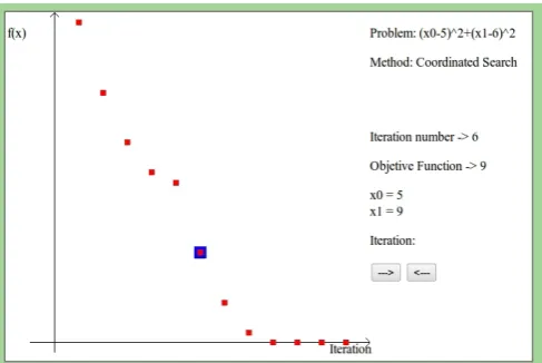
In one of these pages, the user can visualize the various values of the objective function as a function of the iteration number (Fig. 6). To the user is presented a plot with all values of the objective function, and the data for the highlighted element. The user can do a step-by-step visualization of data, changing the selected data element by clicking in the button with the right arrow (next iteration) or the left arrows (previous iteration).

Figure 6. Evolution of the objective function of the problem(x0−5)2+

(x1−6)2, as a function of the iteration number, using the Coordinated

Search method.

For problems in R2 it is also possible to visualize all the intermediate values for the solution (x0 and x1), found by the method at each iteration (Fig. 7). Also in this case it is presented to the user a plot with all values obtained in the execution of the method, and for the highlighted element the corresponding data is presented on the right of the web page. Also a step-by-step analysis of the values is possible in the page.

Figure 7. Some of the approximations to the solutions found by the the Coordinated Search method for problem(x0−5)2+ (x1−6)2, starting

at the initial point(10.0,10.0).

IV. CONCLUSION ANDFUTUREWORK

methods for later analysis. Data can be stored either in the local computer where the API is installed and running, or in a remote server (e.g. using the Internet) as long as there is a possible route between the hosts. Access to the data is made using a standard web browser, allowing users to access and visualization of data without the need to install any application in their computer, independently of the user location and the users’ computing platform.

Future works includes the enhancement and conclusion of a Java-based API for graphical representation, that has also started to be developed, to improve the visual quality of the graphics presented by the developed application.

Also the possibility of generation of a local XML (eXtensi-ble Markup Language), instead of sending data to a database, is to be implemented. This will allow users to generate a local log file, without the need to have access to a database server where to store the data. This XML file can later be sent to an application (which can be the web-based application presented in this paper) for data visualization.

REFERENCES

[1] A. R. Conn, K. Scheinberg, and L. N. Vicente, Introduction to Derivative-Free Optimization. Philadelphia, USA: MPS-SIAM Series on Optimization, SIAM, (2009).

[2] R. Lewis, V. Torczon, and M. Trosset, “Direct search methods: Then and now,”J. Comput. Appl. Math., no. 124, pp. 191–207, (2000). [3] T. Kolda, R. Lewis, and V. Torczon, “Optimization by direct search:

New perspectives on some classical and modern methods,” SIAM Review, vol. 45, pp. 385–482, (2003).

[4] R. Hooke and T. Jeeves, “Direct search solution of numerical and statistical problems,”Journal of the Association for Computing Machinery, vol. 8, no. 2, pp. 212–229, (1961).

[5] J. Matias, A. Correia, P. Mestre, C. Fraga, and C. Serˆodio, “Web-based application programming interface to solve nonlinear optimization problems,” inLecture Notes in Engineering and Computer Science -World Congress on Engineering 2010, vol. 3. London, UK: IAENG, (2010), pp. 1961–1966.

[6] A. Correia, J. Matias, P. Mestre, and C. Serˆodio, “Derivative-free Nonlinear Optimization Filter Simplex, International,” Journal of Applied Mathematics and Computer Science (AMCS), vol. 4029, no. 4, pp. 679–688, Dec 2010.

[7] A. Correia, J. Matias, P. Mestre, and C. Serˆodio, “Derivative-free optimization and filter methods to solve nonlinear constrained problems,”International Journal of Computer Mathematics, vol. 86, no. 10, pp. 1841–1851, (2009).

[8] A. Correia, J. Matias, P. Mestre, and C. Serodio, Classification of Some Penalty Methods. Birkh¨auser/Springer, Dec 2009, vol. 2, pp. 131–140.

[9] A. Correia, J. Matias, P. Mestre, and C. Serˆodio, “Direct-search penalty/barrier methods,” in Lecture Notes in Engineering and Computer Science - World Congress on Engineering 2010, vol. 3. London, UK: IAENG, (2010), pp. 1729–1734.

[10] A. Correia, J. Matias, P. Mestre, and C. Serˆodio, “Constrained nonlinear optimization without derivatives,” inProceedings of MATH-MOD 2009 - 6th Vienna International Conference on Mathematical Modelling, (2009), pp. 2499–2503.

[11] A. Correia, “M´etodos de pesquisa directa: Optimizac¸˜ao n˜ao linear,” Ph.D. dissertation, University of Tr´as-os-Montes e Alto Douro, Vila Real, Portugal, (2010).

[12] P. Mestre, J. Matias, A. Correia, and C. Serodio, “Direct Search Op-timization Application Programming Interface with Remote Access,” IAENG International Journal of Applied Mathematics, vol. 40, no. 4, pp. 251–261, Nov 2010.

[13] C. Audet and J. Dennis, “A pattern search filter method for nonlinear programming without derivatives,” SIAM Journal on Optimization, vol. 5, no. 14, pp. 980–1010, (2004).

[14] C. Audet and J. E. D. Jr., “Mesh adaptive direct search algorithms for constrained optimization,”SIAM Journal on Optimization, no. 17, pp. 188–217, (2006).

[15] C. Audet and J. E. D. Jr., “A mads algorithm with a progressive barrier for derivative-free nonlinear programming,” Les Cahiers du GERAD, ´

Ecole Polytechnique de Montr´eal, Tech. Rep. G-2007-37, (2007). [16] J. Dennis and D. Woods, “Optimization on microcomputers: The

nelder-mead simplex algorithm,” New Computing Environments: Microcomputers in Large-Scale Computing,, vol. Wouk, A., ed., pp. 116–122, (1987).

[17] C. Kelley,Iterative Methods for Optimization. Philadelphia, USA: Number 18 in Frontiers in Applied Mathematics, SIAM, (1999). [18] J. Lagarias, J. Reeds, M. Wright, and P. Wright, “Convergence

properties of the nelder–mead simplex method in low dimensions,” SIAM Journal on Optimization, vol. 9, no. 1, pp. 112–147, (1998). [19] P. Tseng, “Fortified-descent simplicial search method: A general

approach,”SIAM Journal on Optimization, vol. 10, no. 1, pp. 269– 288, (2000).

[20] F. Y. Wang and D. Liu, Advances in Computational Intelligence: Theory And Applications (Series in Intelligent Control and Intelligent Automation). River Edge, NJ, USA: World Scientific Publishing Co., Inc., (2006).

[21] X. Hu and R. Eberhart, “Solving constrained nonlinear optimization problems with particle swarm optimization,” in Proceedings of the Sixth World Multiconference on Systemics, Cybernetics and Informatics 2002 (SCI 2002), (2002), pp. 203–206.

[22] S. Zhang, “Constrained optimization byconstrained hybrid algorithm of particle swarm optimization and genetic algoritnm,” inProceedings of AI 2005: Advances in Artificial Intelligence. Springer: Civil-Comp press, (2005), pp. 389–400.

[23] J. Matias, “T´ecnicas de penalidade e barreira baseadas em m´etodos de pesquisa directa e a ferramenta pnl-pesdir,” Ph.D. dissertation, UTAD, Vila Real, (2003).

[24] A. Pereira, “Caracterizac¸˜ao da func¸˜ao de penalidade exponencial num m´etodo de reduc¸˜ao para programac¸˜ao semi-infinita,” Ph.D. dissertation, Universidade do Minho, Braga, (2006).

[25] R. H. Byrd, J. Nocedal, and R. A. Waltz, “Steering exact penalty methods for nonlinear programming,” Optimization Methods & Software, vol. 23, no. 2, pp. 197–213, (2008).

[26] N. I. M. Gould, D. Orban, and P. L. Toint, “An interior-pointl1-penalty

method for nonlinear optimization,” Rutherford Appleton Laboratory Chilton, Tech. Rep., (2003).