An Aggregate Production Plan for a Biscuit Manufacturing Plant Using Integer Linear Programming

(1)

ISSN Online: 2333-9721 ISSN Print: 2333-9705

DOI: 10.4236/oalib.1105743 Nov. 28, 2019 1 Open Access Library Journal

An Aggregate Production Plan for a Biscuit

Manufacturing Plant Using Integer Linear

Programming

Dilishiya Kalpani De Silva, Wasantha Bandara Daundasekara

Department of Mathematics, Faculty of Science, University of Peradeniya, Peradeniya, Sri Lanka

Abstract

Effective planning, scheduling, and synchronization of all production activi-ties are the key responsibiliactivi-ties of the management of a manufacturing plant. Therefore, it is necessary for the management of the plant to design the pro-duction process so that the total propro-duction cost is minimized, subject to the available resources that cannot be compromised. In this study, a biscuit man-ufacturing plant is selected and an integer linear programming (ILP) model is formulated to determine aggregate number of batches that the plant should produce from each product per month so that monthly demand is satisfied with available resources. The objective is to minimize the monthly production cost of the plant. The required data were collected from the production plant for a period of one month, and then, the objective function and constraints were formulated. The management has given a paramount importance in sa-tisfying the demand so that there will not be any unsatisfied customer. Ac-cording to the managerial requirement, any feasible solution obtained by the model must satisfy the demand. Therefore, demand constraint is considered as a hard constraint. The management is forced to adjust the labour and ma-chine requirements more frequently according to the monthly demand. Thus, labour and machine hour constraints are considered as soft constraints. For-mulated ILP model was implemented as a spreadsheet model in Excel and solved using Excel Solver which uses the simplex algorithm and incorporates the integer requirement of the model when finding the optimal solution. To-tal available labour and machine hours can be changed within a particular range until a feasible solution is found. The solved model determines the number of batches to be produced from each product and the corresponding minimum cost per month. By implementing this production plan, manufac-turing excess of biscuits can be avoided and hence utilizes the physical and human resources to the optimum manner. Additionally, the machine and

la-How to cite this paper: De Silva, D.K. and Daundasekara, W.B. (2019) An Aggregate Production Plan for a Biscuit Manufacturing Plant Using Integer Linear Programming. Open Access Library Journal, 6: e5743.

https://doi.org/10.4236/oalib.1105743

Received: August 30, 2019 Accepted: November 25, 2019 Published: November 28, 2019

This work is licensed under the Creative Commons Attribution International License (CC BY 4.0).

http://creativecommons.org/licenses/by/4.0/

(2)

DOI: 10.4236/oalib.1105743 2 Open Access Library Journal

bour idle times and the needed overtime hours can be identified using the solution while the additional overtime cost will be added to the monthly production cost.

Subject Areas

Corporate Governance

Keywords

Integer Linear Programming, Soft Constraints, Hard Constraints, Spreadsheet Model, Excel Solver, Simplex Algorithm

1. Introduction

Proper functioning of a manufacturing plant requires efficient planning, sche-duling, and synchronization of all production activities. Thus, a production plan (PP) is an important part of a business plan that the manufacturing or produc-tion department is responsible for developing. It is necessary for the manage-ment of the plant to determine the total amount of output that the manufactur-ing plant should produce from each period in the plannmanufactur-ing horizon in order to satisfy the customer demand with the limited available resources in the plant. The output is generally expressed in terms of units of measurement such as tons, liters, kilograms and batches. A quantitative solution for the PP problem can be found in different ways. One method is to use a mathematical model to solve a PP problem. The applications of Operations Research (OR) are widely used in industrial sector due to its ability to optimize a given scenario resulting in max-imum possible gain. In practical situations, linear programming is a part of a very essential area of mathematics termed “optimization techniques”. A mathe-matical model can be formulated using linear programming (LP) [1] with the objective of minimizing the cost or maximizing the profit without violating the constraints of limited resources and satisfying the demand constraint in order to determine the number of units to be produced from each item. Tingley [2] re-vealed that LP is a conventionally used technique. However, in order to apply LP to a production planning problem, the data input should be uniquely deter-mined.

(3)

were used, many authors attempted to solve the APP problem. In APP, the aim is to obtain overall (aggregate) production quantities for each product. Other approaches such as goal programming have been used to solve the APP problem in the literature [11] [12] [13]. Since defining goals is a managerial decision, the problem is reduced to a linear programming problem. In real-world APP prob-lems, the input data or parameters, such as demand, resources, cost and objec-tive function are often uncertain (fuzzy) because some information is incomplete or unavailable. Therefore, Fuzziness is included in most models in previous stu-dies to find a solution to APP [7] [8] [14]. Moreover, Wang and Fang [15] in-corporated the fuzzy nature of parameters and presented a fuzzy linear pro-gramming method for solving the APP. However, the data such as cost and re-sources for this study were obtained from the manufacturing plant. The com-plexity of the problem reduces as the monthly demand is decided by the top management and informed the production managers at the beginning of each month. Thus, as mentioned earlier, an LP model can be developed to solve this PP problem considering only one month as the data input is uniquely deter-mined. The aim of this study is to determine the number of batches to be pro-duced from each product per month in order to satisfy the monthly demand with the available resources while minimizing the production cost. Owing to the fact that the plant does not produce partial batches, all the variables are re-stricted to be integers. Thus, in this study, an integer linear programming (ILP) model [16] is used to solve the PP problem. In our mathematical model all the decision variables are restricted to be integers. However, when only a set of va-riables are integers, the problem can be solved using mixed integer linear pro-gramming (MILP) problem [17] [18].

If the plant has the capability of producing biscuits according to the monthly demand, based on their past experience, without using further quantitative ana-lytical methods, then most of the biscuits will remain in the finished-goods stores for a longer period, before they are sent to the warehouses or other distri-buting areas. As a result, more often, by the time customer consumes the prod-uct, biscuits are reaching their expiration date, so that the moisture level of bis-cuits will be increased, the appearance and the colour may have changed, and the crispiness will be reduced. Once such low-quality products are released to the market, the goodwill of the customer regarding the product would be lost. An improved PP for the production plant is extremely important since a better production plan will reduce the time that the finished goods remain in the stores, thus, prevent the additional inventory costs and the quality of the product will be fresh by the time consumer consumes it. In addition, the product can be sent to the market according to the demand without unnecessary delays.

(4)

[image:4.595.276.472.308.709.2]

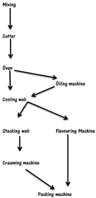
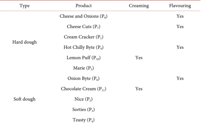
DOI: 10.4236/oalib.1105743 4 Open Access Library Journal Figure 1 for the production process). The plant is producing various types of products, which are mainly categorized as soft dough and hard dough biscuits. In addition, there are certain products, which are unique and need further man-ufacturing process such as oiling, creaming and flavouring. These deviations are taken into account when the mathematical model is formulated. The range of products that are produced in the plant is presented in Table 1. The table cate-gorises the products as soft dough and hard dough and specifies the biscuits which use the additional processing; creaming and flavouring. Furthermore, the coefficients for both objective function and constraints are calculated to develop the mathematical model by considering the process of the biscuit plant.

2. Materials and Methods

A mathematical model to determine the number of batches to be produced from each item (see Table 1 for all the available products in this plant) was formu-lated using ILP with the objective of minimizing the cost without violating the

(5)

[image:5.595.210.541.89.294.2]

Table 1. Range of products.

Type Product Creaming Flavouring

Hard dough

Cheese and Onions (P8) Yes

Cheese Cuts (P7) Yes

Cream Cracker (P1)

Hot Chilly Byte (P9) Yes

Lemon Puff (P10) Yes

Marie (P5)

Soft dough

Onion Byte (P6) Yes

Chocolate Cream (P11) Yes

Nice (P2)

Sorties (P3)

Teasty (P4)

constraints of limited resources and satisfying the demand constraint. All the necessary data were collected and the coefficients corresponding to the objective and constraints were estimated as demonstrated in the following sections.

2.1. Formulating the Mathematical Model

Let xi be the number of batches to be produced from the ith product (Pi) per

month, where i=1,2, ,11_ _. 2.1.1. Objective

The objective is to minimize the monthly manufacturing cost of unpacked bis-cuits (baked bisbis-cuits, which are not packed but stacked into the bins). The pro-duction cost per kilogram of biscuits for unpacked biscuit was collected as raw data. It involves raw material cost, labour cost, fuel cost for the oven, electricity etc. After incorporating these costs, the objective function was formulated as follows:

Let Ci be the production cost per finished batch of the ith product.

11 1

minZ =

∑

i=C x OCi i+ ;

where Ci is the cost per batch of the ith product and OC is the overtime cost.

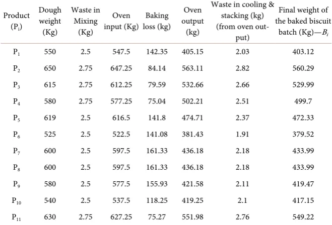
The wastage produced in the process of biscuit manufacturing and weight losses at each section are illustrated in Table 2. Afterward, all the wastages and weight losses mentioned in Table 2 were reduced from the weight of the wet dough mixture. The model is developed and solved assuming that these are the only wastages that will occur in the production process. All the necessary data are exhibited in Table 3. It enumerates the weight of a baked biscuit batch (Bi).

Given that the cost per kilogram (ki) was collected as raw data, the cost per batch

of the ith_{product (}_C

i) can be calculated using the following formulas. The

(6)

[image:6.595.208.540.104.335.2]

Table 2. The wastage produced in the process of biscuit manufacturing and weight losses at each section.

Product (Pi) Dough Weight _(Kg) Baking _{loss %} Waste at mixing _(kg) Waste at cutter _(kg)

Waste in cooling & stacking % (from

oven output)

P1 550 26 1 1.5 0.5

P2 650 13 0.75 2 0.5

P3 615 13 0.75 2 0.5

P4 580 13 0.75 2 0.5

P5 619 23 1 1.5 0.5

P6 525 27 1 1.5 0.5

P7 600 27 1 1.5 0.5

P8 600 27 1 1.5 0.5

P9 580 27 1 1.5 0.5

P10 540 22 1 1.5 0.5

[image:6.595.209.539.366.590.2]

P11 630 12 0.75 2 0.5

Table 3. Weights of baked biscuit batches.

Product (Pi)

Dough weight (Kg)

Waste in Mixing

(Kg)

Oven

input (Kg) loss (kg) Baking Oven output

(kg)

Waste in cooling & stacking (kg) (from oven

out-put)

Final weight of the baked biscuit

batch (Kg)—Bi

P1 550 2.5 547.5 142.35 405.15 2.03 403.12

P2 650 2.75 647.25 84.14 563.11 2.82 560.29

P3 615 2.75 612.25 79.59 532.66 2.66 529.99

P4 580 2.75 577.25 75.04 502.21 2.51 499.7

P5 619 2.5 616.5 141.8 474.71 2.37 472.33

P6 525 2.5 522.5 141.08 381.43 1.91 379.52

P7 600 2.5 597.5 161.33 436.18 2.18 433.99

P8 600 2.5 597.5 161.33 436.18 2.18 433.99

P9 580 2.5 577.5 155.93 421.58 2.11 419.47

P10 540 2.5 537.5 118.25 419.25 2.1 417.15

P11 630 2.75 627.25 75.27 551.98 2.76 549.22

Table 4. Cost per batch for each product.

Product (Pi) _{per kilogram (Rs)—K}Production cost i

Final weight of the

baked biscuit batch (Kg)—Bi Cost per batch (Rs)—Ci

P1 150.0015876 403.12 60,468.64

P2 133.000464 560.29 74,518.83

P3 117.0009245 529.99 62,009.32

[image:6.595.209.541.629.736.2]

(7)

Continued

P5 124.0003811 472.33 58,569.1

P6 149.9991568 379.52 56,927.68

P7 260.0024655 433.99 112,838.47

P8 220.0020968 433.99 95,478.71

P9 129.9991179 419.47 54,530.73

P10 170.0015342 417.15 70,916.14

[image:7.595.210.542.237.620.2]

P11 180.0000364 549.22 98,859.62

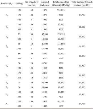
Table 5. Total demand for each product.

Product (Pi) SKU (g) No of packets _{in a box} _{(in boxes)}Demand _{different SKUs (kg)}Total demand for Total demand for each _{product type (Kg)}

P1

125 50 1475 9218.75

19,769

190 24 1875 8550

500 4 1000 2000

P2

100 50 2500 12,500

15,500

500 4 1500 3000

P3

75 50 47,500 178,125

19,200

320 4 15,000 19,200

P4

60 50 45,000 135,000

21,000

300 4 17,500 21,000

P5

80 50 4250 17,000

18,050

300 4 875 1050

P6

30 20 8750 5250

10,320

130 20 1950 5070

P7

170 24 2250 9180

12,015

210 10 1350 2835

P8 25 20 22,500 11,250 11,250

P9 30 20 20,000 12,000 12,000

P10

100 48 2150 10,320

17,520

200 24 1500 7200

P11

100 50 2625 13,125

14,725

400 4 1000 1600

Dough Weight Waste in Mixing Baking Loss Waste in Cooling &Stacking

i

B = − −

−

( )

Production cost per kilogram of biscuits Weight of a baked biscuit batch

i i

i

C K

B

=

× .

(8)

1 2 3 4

5 6 7 8

9 10 11

min 60468.64 74518.83 62009.32 57964.79 58569.10 56927.68 112838.47 95478.71 54530.73 70916.14 98859.62

Z x x x x

x x x x

x x x

= + + +

+ + + +

+ + +

.

2.1.2. Constraints

Satisfying all constraints is essential for the feasibility. However, many models contain two categories of constraints: hard constraints that must be satisﬁed by any feasible solution and the soft constraints of different relative importance may or may not be satisﬁed. Hvolby and Steger-Jensen [19] discussed using soft constraints and hard constraints in production planning. The hard constraints stipulate the set of feasible solutions, and the soft constraints stipulate a function to be optimized in deciding between the feasible solutions. If both kinds of con-straints exist in a model, soft concon-straints can be adjusted, until a feasible solution is found.

1) Hard Constraint

• _{Demand constraint}

The management has given utmost importance in satisfying the demand so that there will not be any unsatisfied customer. Any feasible solution obtained by the model must satisfy the demand. Therefore, for this study, demand constraint was considered as a hard constraint.

Since xi is the number of batches to be produced from the ithproduct, Bixi

gives the total number of kilograms that have to be produced from the ith

prod-uct per month. This amount should be equal to the demand of each prodprod-uct (in kilograms) to satisfy the demand as the plant does not want to produce any excess amount of biscuits. Thus, the demand constraint, in general, can be writ-ten as follows:

i i i

B x ≥D_for i=1,2, ,11 ;

where Di is the monthly demand in kilograms for the ith product.

The monthly demand is decided by the top management which is passed away to the biscuit plant at the beginning of every month. The demand is expressed as the number of boxes of biscuits needed for different stock keeping units (SKU) from each product. These data were collected from the manufacturing plant and monthly demand in kilograms for each product was calculated utilizing these data. Table 5 enumerates all the necessary calculations to find the total demand in kilograms per month from each product.

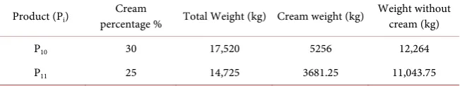
As illustrated in Table 1, the product types, Lemon Puff (P10) and Chocolate

[image:8.595.213.539.663.724.2]

cream (P11) have a cream layer. Thus, in Table 6, the cream weight was reduced

Table 6. Biscuit weight without cream.

Product (Pi) _{percentage %}Cream Total Weight (kg) Cream weight (kg) Weight without _{cream (kg)}

P10 30 17,520 5256 12,264

(9)

from the total demand which was calculated in Table 5 for P10 and P11 in order

to calculate the total amount of baked biscuits that should be produced.

After calculating all the coefficient values and right-hand side values which are the requirements, the demand constraints for each product can be written as follows:

1

403.12425x ≥19769

2

560.2919625x ≥15500

3

529.9942125x ≥19200

4

499.6964625x ≥21000

5

472.331475x ≥18050

6

379.517875x ≥10320

7

433.994125x ≥12015

8

433.994125x ≥11250

9

419.467125x ≥12000

10

417.15375x ≥12264

11

549.2201x ≥11043.75_.

2) Soft Constraints

The manufacturing company has limited amount of resources. Therefore, it is essential to consider available resources in the plant when minimizing the man-ufacturing cost. When the biscuits are manufactured, manman-ufacturing process cannot exceed consuming the available amount of resources such as the number of labourers and the machine capacity. The management is repeatedly adjusting the labour and machine requirements according to the monthly demand. Thus, in this study, labour and machine hour constraints were considered as soft con-straints.

• _{Machine Hours}

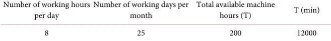
A batch of each product takes a certain processing time. The required total processing time for the monthly production should be less than or equal to total available machine hours per month. If the demand cannot be satisfied with the available total machine hours, number of working hours per day and working days per month can be increased up to some level in the model solving step. Therefore, machine hour constraint was considered as a soft constraint. Then, the machine hour constraint, in general, is as follows:

11 1 i i i=t x T≤

∑

for i=1,2, ,11_ _,

where ti is the total processing time (in minutes) per batch of the ith product and

T is the available machine time (in minutes) per month.

(10)

[image:10.595.209.538.94.135.2]

Table 7. Available machine hours per month.

Number of working hours

per day Number of working days per month Total available machine hours (T) T (min)

8 25 200 12000

1 2 3 4 5 6 7

8 9 10 11

30 25 20 26 40 50 45

50 50 30 30 12000

x x x x x x x

x x x x

+ + + + + +

+ + + + ≤ .

• _{Labor hour constraint}

The required labour hours for the monthly production should be less than the available labour hours per month. Thus, the labour hour constraint for each sec-tion; mixing, cutter, baking and cooling, and stacking can be formulated, in general, as follows:

11 1 i I i i=t l x L≤

∑

,

for each of the four sections mixing, cutter, baking and cooling, and stacking, where li is the number of labourers needed for each production section, ti is the

processing time (in minutes) per batch of the ith_{product through each section}

and L is the total available labour hours.

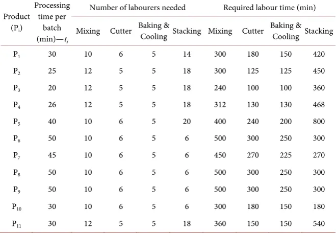
A fixed number of labourers are allocated to each section of the production plant (see Table 8). Among these labourers, different numbers of labourers are assigned into each section during the production of different products (see Ta-ble 9). Moreover, the calculations of the required labour time for each section during the production are demonstrated in Table 9 and the available labour time in minutes is shown in Table 8.

Since the number of working days or hours can be adjusted until a feasible solution is found, this constraint is also identified as a soft constraint. Therefore, labour constraint for each section for this PP problem can be presented as follows:

Mixing:

1 2 3 4 5 6 7

8 9 10 11

300 300 240 312 400 500 450

500 500 300 360 144000

x x x x x x x

x x x x

+ + + + +

+ + + + ≤

+

.

Cutter:

1 2 3 4 5 6 7

8 9 10 11

180 125 100 130 240 300 270

300 300 180 150 72000

x x x x x x x

x x x x

+ + + + + +

+ + + + ≤ .

Baking and Cooling:

1 2 3 4 5 6 7

8 9 10 11

150 125 100 130 200 250 225

250 250 150 150 72000

x x x x x x x

x x x x

+ + + + + +

+ + + + ≤ .

Stacking:

1 2 3 4 5 6 7

8 9 10 11

420 450 360 468 800 300 270

300 300 180 540 240000

x x x x x x x

x x x x

+ + + + +

+ + + + ≤

+

.

In addition, all the xi values should be positive integers as the plant does not

(11)

Table 8. Number of labours assigned for each section and available labour hours per month.

Section Available number _{of labours} Number of _days Number of _hours L (h) L (min)

Mixing 12 25 8 2400 144,000

Cutter 6 25 8 1200 72,000

Baking and Cooling 5 25 8 1200 72,000

[image:11.595.211.539.103.199.2]

Stacking 20 25 8 4000 240,000

Table 9. Required labour time.

Product (Pi)

Processing time per

batch (min)—ti

Number of labourers needed Required labour time (min)

Mixing Cutter Baking & _{Cooling Stacking Mixing Cutter} Baking & _{Cooling Stacking}

P1 30 10 6 5 14 300 180 150 420

P2 25 12 5 5 18 300 125 125 450

P3 20 12 5 5 18 240 100 100 360

P4 26 12 5 5 18 312 130 130 468

P5 40 10 6 5 20 400 240 200 800

P6 50 10 6 5 6 500 300 250 300

P7 45 10 6 5 6 450 270 225 270

P8 50 10 6 5 6 500 300 250 300

P9 50 10 6 5 6 500 300 250 300

P10 30 10 6 5 6 300 180 150 180

P11 30 12 5 5 18 360 150 150 540

2.2. Solving the Formulated Mathematical Model

The most prominent algorithm to solve LP problems is the Simplex Algorithm developed by Dantzig in 1947. However, the formulated model has integer deci-sion variables and therefore it is referred to as Integer Linear Programming (ILP). Thus, the problem cannot be solved using the simplex method alone. One class of exact algorithms that can be used to solve ILP is cutting plane methods

[20]. This method first uses LP relaxation and afterward adds linear constraints so that it will lead the solution towards being integer without excluding any in-teger feasible points. Another class of exact algorithms is variants of the branch and bound method [21]. Many problems are intractable since ILP is NP-hard (see [22]), thus heuristic methods are used instead. Hill climbing (see [23]), si-mulated annealing (see [24]), and ant colony optimization (see [25]) are some of the heuristic methods that can be applied to solve ILPs. However, in this study spreadsheet paradigm was used to solve the formulated ILP problem.

Model in Microsoft Excel

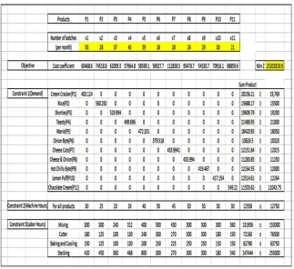
[image:11.595.209.539.233.462.2]

(12)

Excel (see Figure 2). Major spreadsheet packages come with a built-in optimiza-tion tool called Solver. MacDonald [26] explained how to use Microsoft Excel Solver to solve LP problems. Many authors in the literature have used the Excel Solver to solve different linear and integer linear programming problems [27] [28]. Once a model was implemented in a spreadsheet, the optimal values of the decision variables and the optimal objective function value can be found using Excel Solver. In the Solver dialog box, Simplex LP was selected to solve the ILP implemented in Excel as a spreadsheet model, where Solver uses a Branch and Bound to solve the model. The demand constraint should be satisfied by any so-lution of this problem as it was identified as a hard constraint. The number of working hours, working days were changed within a particular range acceptable to the management, and a feasible solution was found when the number of working hours was increased up to 8.5 hours, while number of labours assigned for each section considered constant. Since the production process is continuous, labourers and machines in all sections should work for additional 0.5 hours. As a result, the right-hand side of the machine hour and labour hour constraint were changed as displayed in the spreadsheet model in Figure 2. The overtime cost can be calculated separately, thus, it is not included in the spreadsheet model.

3. Results and Discussion

3.1. Results

[image:12.595.212.536.413.709.2]

According to the obtained optimum solution, the number of batches to be

(13)

produced from each product per month is displayed in Figure 2, and according to Figure 2, monthly demand can be satisfied using the available resources with a minimum cost of approximately Rs.25.2 million. In order to achieve that, the plant should produce following number of batches from each product:

x1 (Cream Cracker) = 50, x2 (Nice) = 28, x3 (Sorties) = 37, x4 (Teasty) = 43, x5

(Marie) = 39, x6 (Onion byte) = 28, x7 (Cheese cuts) = 28, x8 (Cheese and Onion)

= 26, x9 (Hot chilly Byte) = 29, x10 (Lemon Puff) = 30, x11 (Chocolate Cream) =

21.

Moreover, in order to satisfy the customer demand, the manufacturing plant should function 25 days and 8.5 hours continuously each day for this particular month.

3.2. Discussion

The Excel does not provide sensitivity report, as the variables are integers. Therefore, sensitivity analysis cannot be performed for the optimal solution. The total monthly cost can be reduced by Rs. 474,705 if the integer constraint is re-moved and this additional monthly cost is due to the excess amount of biscuits that will be produced due to the integer constraint. Consequently, if the compa-ny can produce partial batches, then the monthly additional cost of producing additional biscuits could be reduced and the excess amount of biscuits produced could be avoided.

In addition, the solved model (using sum product column) identifies the number of working hours and working days of the production plant per month and the total kilograms of biscuits from each product should be produced by the end of month. However, the minimum number of hours that the plant should function to get a feasible solution is 8.372 hours. However, it was round up to 8.5 considering the convenience of paying overtime. If we assume that all the 43 la-bourers are working 8.5 hours for all the 25 days even though for some products some labourers are kept idle, the overtime cost will be (8.5 − 8) × 25 × 43 × OTR, where OTR is the overtime rate. Moreover, idle times of labourers and machines can be obtained by observing the spreadsheet model.

Even though this study was carried out based on the data of a particular month, this model can be generalized to determine the number of batches to be produced for any month. As Di’s are changing from month to month, applying

new Di’s to the formulated spreadsheet model would give the number of

prod-ucts to be produced in each month. In addition, number of working hours and working days can be appropriately changed in the model until it reaches feasibil-ity.

(14)

4. Conclusions

Based on the results obtained above, the solved integer linear programming model gives a feasible solution and it minimizes the monthly manufacturing cost. It could be concluded that by implementing the production plan suggested by the solution, the monthly demand could be satisfied using the available re-sources while minimizing the monthly production cost.

Moreover, the management can schedule the production for each day, as the aggregate number of batches to be produced for each product and the numbers of labour hours needed for the month are predetermined. If the plant overpro-duced the biscuits, the biscuits would be remained in the finished goods stores for an additional period, which results in excessive amount of inventory cost. This will also lead to low quality products entering into the market, causing bad reputation to the production plant. Therefore, by implementing this production plan, manufacturing excess of biscuits can be avoided and hence utilizes the physical and human resources to the optimum manner. This will enable manu-facturing plant to reduce the production cost. Moreover, using the proposed mathematical model and with the help of Excel spreadsheet, the company can plan the production for the coming years.

Conflicts of Interest

The authors declare no conflicts of interest regarding the publication of this pa-per.

References

[1] Kantorovich, L.V. (1939) The Mathematical Method of Production Planning and Organization. Management Science, 6, 363-422.

[2] Tingley, G.A. (1987) Can MS/OR Sell Itself Well Enough? Interfaces, 17, 41-52.

https://doi.org/10.1287/inte.17.4.41

[3] Hanssmann, F. and Hess, S.W. (1960) A Linear Programming Approach to Produc-tion and Employment Scheduling. Management Science, 1, 46-51.

https://doi.org/10.1287/mantech.1.1.46

[4] Hung, Y.F. and Leachman, R.C. (1996) A Production Planning Methodology for Semiconductor Manufacturing Based on Iterative Simulation and Linear Program-ming Calculations. IEEE Transactions on Semiconductor Manufacturing, 9, 257-269. https://doi.org/10.1109/66.492820

[5] Pendharkar, P.C. (1997) A Fuzzy Linear Programming Model for Production Plan-ning in Coal Mines. Computers&OperationsResearch, 24, 1141-1149.

https://doi.org/10.1016/S0305-0548(97)00024-5

[6] Vasant, P.M. (2003) Application of Fuzzy Linear Programming in Production Plan-ning. FuzzyOptimizationandDecisionMaking, 2, 229-241.

https://doi.org/10.1023/A:1025094504415

[7] Wang, R.C. and Liang, T.F. (2004) Application of Fuzzy Multi-Objective Linear Programming to Aggregate Production Planning. Computers & Industrial Engi-neering, 46, 17-41.https://doi.org/10.1016/j.cie.2003.09.009

(15)

Aggregate Production Planning. Internationaljournalofproductioneconomics, 98, 328-341.https://doi.org/10.1016/j.ijpe.2004.09.011

[9] Kanyalkar, A.P. and Adil, G.K. (2005) An Integrated Aggregate and Detailed Plan-ning in a Multi-Site Production Environment Using Linear Programming. Interna-tionalJournalofProductionResearch, 43, 4431-4454.

https://doi.org/10.1080/00207540500142332

[10] da Silva, C.G., Figueira, J., Lisboa, J. and Barman, S. (2006) An Interactive Decision Support System for an Aggregate Production Planning Model Based on Multiple Criteria Mixed Integer Linear Programming. Omega, 34, 167-177.

https://doi.org/10.1016/j.omega.2004.08.007

[11] Goodman, D.A. (1974) A Goal Programming Approach to Aggregate Planning of Production and Work Force. ManagementScience, 20, 1569-1575.

https://doi.org/10.1287/mnsc.20.12.1569

[12] Jamalnia, A. and Soukhakian, M.A. (2009) A Hybrid Fuzzy Goal Programming Ap-proach with Different Goal Priorities to Aggregate Production Planning. Computers &IndustrialEngineering, 56, 1474-1486.https://doi.org/10.1016/j.cie.2008.09.010

[13] Leung, S.C. and Chan, S.S. (2009) A Goal Programming Model for Aggregate Pro-duction Planning with Resource Utilization Constraint. Computers & Industrial Engineering, 56, 1053-1064.https://doi.org/10.1016/j.cie.2008.09.017

[14] Masud, A.S. and Hwang, C.L. (1980) An Aggregate Production Planning Model and Application of Three Multiple Objective Decision Methods. InternationalJournalof ProductionResearch, 18, 741-752.https://doi.org/10.1080/00207548008919703

[15] Wang, R.C. and Fang, H.H. (2001) Aggregate Production Planning with Multiple Objectives in a Fuzzy Environment. European Journal of Operational Research, 133, 521-536.https://doi.org/10.1016/S0377-2217(00)00196-X

[16] Wolsey, L.A. (1998) Integer Programming. Wiley, New York.

[17] Orcun, S., Altinel, I.K. and Hortaçsu, Ö. (2001) General Continuous Time Models for Production Planning and Scheduling of Batch Processing Plants: Mixed Integer Linear Program Formulations and Computational Issues. Computers &Chemical Engineering, 25, 371-389.https://doi.org/10.1016/S0098-1354(00)00663-3

[18] Floudas, C.A. and Lin, X. (2005) Mixed Integer Linear Programming in Process Scheduling: Modeling, Algorithms, and Applications. Annals of Operations Re-search, 139,131-162.https://doi.org/10.1007/s10479-005-3446-x

[19] Hvolby, H.H. and Steger-Jensen, K. (2010) Technical and Industrial Issues of Ad-vanced Planning and Scheduling (APS) Systems. Computers in Industry, 61, 845-851.https://doi.org/10.1016/j.compind.2010.07.009

[20] Gomory, R.E. (1963) An Algorithm for Integer Solutions to Linear Programs. Re-centAdvancesinMathematicalProgramming, 64, 260-302.

[21] Land, A. and Doig, A. (1960) An Automatic Method of Solving Discrete Program-ming Problems. Ecometrics, 28, 497-520.https://doi.org/10.2307/1910129

[22] Schrijver, A. (1998) Theory of Linear and Integer Programming. John Wiley & Sons, New York.

[23] Beale, E.M.L. (1985) Integer Programming. Computational Mathematical Pro-gramming, 15, 1-24. https://doi.org/10.1007/978-3-642-82450-0_1

[24] Abramson, D. and Randall, M. (1999) A Simulated Annealing Code for General In-teger Linear Programs. AnnalsofOperationsResearch, 86, 3-21.

https://doi.org/10.1023/A:1018915104438

(16)

Ant Colony Optimization with ILP Preprocessing in Multiobjective Project Portfo-lio Selection. EuropeanJournalofOperationalResearch, 171, 830-841.

https://doi.org/10.1016/j.ejor.2004.09.009

[26] MacDonald, Z. (1995) Teaching Linear Programming Using Microsoft Excel Solver.

ComputersinHigherEducationEconomicsReview, 9, 7-10.

[27] Trick, M.A. (2004) Using Sports Scheduling to Teach Integer Programming. INFORMS TransactionsonEducation, 5, 10-17.https://doi.org/10.1287/ited.5.1.10