Alan W. F. Boyd
A Thesis Submitted for the Degree of PhD at the
University of St. Andrews
2010
Full metadata for this item is available in Research@StAndrews:FullText
at:
https://research-repository.st-andrews.ac.uk/
Please use this identifier to cite or link to this item: http://hdl.handle.net/10023/1295
This item is protected by original copyright
Node Reliance: An Approach to Extending
the Lifetime of Wireless Sensor Networks
A thesis to be submitted to the
UNIVERSITY OF ST ANDREWS
for the degree of
DOCTOR OF PHILOSOPHY
by
Alan W. F. Boyd
School of Computer Science
University of St Andrews
Abstract
A Wireless Sensor Network (WSN) consists of a number of nodes, each typically having
a small amount of non-replenishable energy. Some of the nodes have sensors, which may
be used to gather environmental data. A common network abstraction used in WSNs is the
(source, sink) architecture in which data is generated at one or more sources and sent to
one or more sinks using wireless communication, possibly via intermediate nodes.
In such systems, wireless communication is usually implemented using radio. Transmitting
or receiving, even on a low power radio, is much more energy-expensive than other
activ-ities such as computation and consequently, the radio must be used judiciously to avoid
unnecessary depletion of energy. Eventually, the loss of energy at each node will cause it
to stop operating, resulting in the loss of data acquisition and data delivery. Whilst the loss
of some nodes may be tolerable, albeit undesirable, the loss of certain critical nodes in a
multi-hop routing environment may cause network partitions such that data may no longer
be deliverable to sinks, reducing the usefulness of the network.
This thesis presents a new heuristic known as node relianceand demonstrates its efficacy in prolonging the useful lifetime of WSNs. The node reliance heuristic attempts to keep as
many sources and sinks connected for as long as possible. It achieves this using areliance valuethat measures the degree to which a node is relied upon in routing data from sources to sinks. By forming routes that avoid high reliance nodes, the usefulness of the network
may be extended.
I, Alan W. F. Boyd, hereby certify that this thesis, which is approximately 78,843 words in
length, has been written by me, that it is the record of work carried out by me, and that it
has not been submitted in any previous application for a higher degree.
date signature of candidate
I was admitted as a research student in October 2005 and as a candidate for the degree
of Doctor of Philosophy in October 2005; the higher study for which this is a record was
carried out in the University of St Andrews between October 2005 and June 2010.
date signature of candidate
I hereby certify that the candidate has fulfilled the conditions of the Resolution and
Regu-lations appropriate for the degree of Doctor of Philosophy in the University of St Andrews
and that the candidate is qualified to submit this thesis in application for that degree.
date signature of supervisor
In submitting this thesis to the University of St. Andrews I understand that I am giving
permission for it to be made available for use in accordance with the regulations of the
University Library for the time being in force, subject to any copyright vested in the work
not being affected thereby. I also understand that the title and abstract will be published,
and that a copy of the work may be made and supplied to anybona fidelibrary or research worker, that my thesis will be electronically accessible for personal or research use unless
exempt by award of an embargo as requested below, and that the library has the right to
migrate my thesis into new electronic forms as required to ensure continued access to the
thesis. I have obtained any third-party copyright permissions that may be required in order
to allow such access and migration, or have requested the appropriate embargo below.
The following is an agreed request by candidate and supervisor regarding the electronic
publication of this thesis: Access to printed copy and electronic publication of thesis
through the University of St Andrews.
Acknowledgements
There are many people without whom this thesis may not have even got off the ground and
to whom I shall owe eternal gratitude:
Dharini Balasubramaniam, my main supervisor, for being forced to put up with endless
proof reads, barely comprehensible musings and endlessly correcting my use of ”in to” as
two words. I am most grateful for her infinite patience, which is more than I deserved.
Alan Dearle and Ron Morrison for acting, at different times, as my second supervisor as
well as having steered the DIAS project on which my studentship was based.
My parents, Ann and Ian Boyd, have provided emotional and financial assistance. Their
academic backgrounds have been invaluable in seeing things from a different perspective.
Claire Loptson, my wonderful girlfriend, for tolerating my daily rants and me in general
and also for making life significantly more bearable than it might otherwise be.
Frank Gunn-Moore and Ali Khajeh-Hosseini for in-car entertainment between Edinburgh
and St Andrews and for bravely proof reading my thesis, despite its size.
Angus Macdonald, Jon Lewis and Jamie Smith for tolerating my daily renditions of the
Wallace & Gromit theme tune.
Kris Getchell, Andrew Gray, Ben Maydon, David Forester, Dawn Fulton, Juliette Daigre,
Gemma McLean, Paula Whiscombe, Keith McDonald, Monika Vorberg, Markus Tauber
and Stuart Norcross for welcome distractions and advice.
Lastly, I wish to thank you, the person I inevitably forgot, who still read my thesis to see if
they’re mentioned in the acknowledgements. Alas, I was time constrained during my final
Published Research
Alan W. F. Boyd, Dharini Balasubramaniam, Alan Dearle, and Ron Morrison.
An approach to extending the lifetime of wireless sensor networks.
InThe 9th Annual PostGraduate Symposium on The Convergence of Telecommunications, Networking and Broadcasting, pages 123–128, Liverpool, UK, 2008.
Alan W. F. Boyd, Dharini Balasubramaniam, Alan Dearle, and Ron Morrison.
On the selection of connectivity-based metrics for wsns using a classification of application
behaviour.
InIEEE International Conference on Sensor Networks, Ubiquitous, and Trustworthy Com-puting, Newport Beach, California, USA (accepted for publication), 2010.
Alan W. F. Boyd, Dharini Balasubramaniam, and Alan Dearle.
A collaborative wireless sensor network routing scheme for reducing energy wastage.
Contents
List of Figures ix
List of Tables xv
1 Introduction 1
1.1 Wireless Sensor Networks . . . 2
1.2 Routing Protocols . . . 2
1.3 Motivation and Problem Statement . . . 3
1.4 Assumptions . . . 5
1.5 Approach: Node Reliance . . . 5
1.6 Contributions . . . 6
1.7 Thesis Structure . . . 7
2 Wireless Sensor Networks 9 2.1 Overview . . . 9
2.2 Relationship to Wireless Ad Hoc Networks . . . 12
2.3 Advantages . . . 12
2.4 Example Deployments . . . 14
2.5 Assumptions . . . 16
2.5.1 Battery Drain from Computation . . . 17
2.5.2 Imperfect Communication . . . 18
2.5.2.1 Unreliability . . . 18
2.5.2.2 Unidirectional Links . . . 20
2.5.3 Mobility . . . 21
2.5.4 Scavenging and Replenishment . . . 21
2.6 Summary . . . 22
3 A Modularised View of Routing Protocols 25
3.1 Discovery . . . 26
3.1.1 Initiator . . . 26
3.1.1.1 Source . . . 26
3.1.1.2 Sink . . . 27
3.1.1.3 Intermediate . . . 27
3.1.2 Preparation . . . 27
3.1.2.1 Proactive Routing . . . 28
3.1.2.2 Reactive Routing . . . 28
3.1.3 Search Method . . . 28
3.1.3.1 Local Knowledge . . . 29
3.1.3.2 Distance Vector . . . 29
3.1.3.3 Global Knowledge (GK) . . . 30
3.1.3.4 Enumeration . . . 31
3.1.4 Table Entries . . . 32
3.1.4.1 Source Full Path . . . 32
3.1.4.2 All Full Path . . . 33
3.1.4.3 Next Hop . . . 33
3.1.5 Summary . . . 34
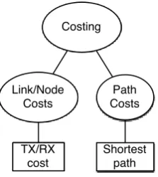
3.2 Costing . . . 34
3.2.1 Link/Node Cost . . . 35
3.2.1.1 Unit . . . 35
3.2.1.2 Geographic Distance . . . 35
3.2.1.3 TX/RX Costs . . . 36
3.2.1.4 Energy Reserves . . . 37
3.2.1.5 Quality of Service . . . 37
3.2.2 Path Costs . . . 38
3.2.2.1 Shortest Path . . . 38
3.2.2.2 Lexicographic Ordering . . . 39
3.2.2.3 Min/Max Element . . . 40
3.2.3 Summary . . . 40
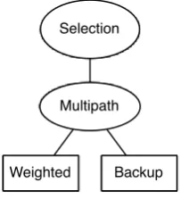
3.3 Selection . . . 41
3.3.1 Topology . . . 41
iii
3.3.1.2 Tree . . . 43
3.3.1.3 Role Assignment . . . 44
3.3.2 Multipath Routing . . . 45
3.3.2.1 Weighted Cost . . . 45
3.3.2.2 Backup Paths . . . 46
3.3.3 Summary . . . 47
3.4 Summary . . . 47
4 Routing Protocols 49 4.1 Classifying Routing Protocols . . . 49
4.2 Minimum Hop Routing . . . 51
4.3 Hierarchical Routing . . . 58
4.4 Geographical Routing . . . 61
4.5 Load Balancing Routing . . . 65
4.5.1 Energy Aware Routing . . . 65
4.5.2 Load Balanced Routing Trees . . . 69
4.5.3 Congestion Adaptive Routing . . . 71
4.6 Minimum Energy Routing . . . 73
4.7 Flow Control . . . 76
4.8 Multipath Routing . . . 78
4.9 Comparison . . . 81
4.10 Summary . . . 85
5 Measuring Source Diversity 87 5.1 Common WSN Metrics . . . 87
5.1.1 Total Data Transfer . . . 89
5.1.2 k-of-n Lifetime . . . 91
5.1.3 Sink Connectivity . . . 91
5.1.4 Triple of (connectivity, number of functional nodes, coverage) . . . 92
5.1.5 Sensor Coverage and Connectivity . . . 93
5.1.6 Conclusions . . . 93
5.2 Connectivity Weighted Transfer . . . 94
5.2.1 Definition of Connection . . . 94
5.2.2 Metric Theory . . . 94
5.2.4 Weighting Factor . . . 96
5.2.5 Operational Concerns . . . 97
5.2.5.1 Effect of Frame Length . . . 98
5.2.5.2 Delay Tolerant Networks . . . 99
5.2.5.3 Continuous Data Streams . . . 99
5.2.5.4 Event and Query-based Systems . . . 100
5.2.5.5 Data Aggregation . . . 100
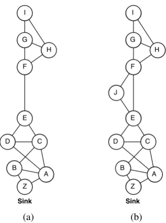
5.2.6 Example . . . 101
5.2.7 Conclusion . . . 103
5.3 Experimental Methodology . . . 104
5.3.1 Algebraic Models . . . 104
5.3.2 Physical Deployments . . . 105
5.3.3 Simulation . . . 105
5.3.4 Chosen Methodology . . . 106
5.4 Simulator Configuration . . . 108
5.4.1 Node Connectivity . . . 108
5.4.2 MAC Protocol . . . 109
5.4.3 Communications Energy . . . 110
5.4.4 Handling Multiple Networks . . . 111
5.4.4.1 Normalising Scores . . . 112
5.4.4.2 Standard Deviation . . . 113
5.5 Summary . . . 113
6 Node Reliance Heuristic 115 6.1 Link/Node Costs . . . 116
6.1.1 Unsuitable Models . . . 118
6.1.1.1 Node Degree . . . 118
6.1.1.2 Clustering Coefficient . . . 119
6.1.1.3 Shortest Paths . . . 121
6.1.1.4 PageRank . . . 122
6.1.1.5 Link Criticality . . . 123
6.1.1.6 Node-Disjoint Paths . . . 124
6.1.1.7 Conclusion . . . 125
6.1.2 Simple Paths Model . . . 125
v
6.1.2.2 Worst-Case Growth Rate . . . 129
6.1.3 Simplest Paths Model . . . 132
6.1.3.1 Example . . . 134
6.1.3.2 Worst-Case Growth Rate . . . 136
6.1.3.3 Advantages . . . 142
6.1.4 Contraction Model . . . 142
6.1.4.1 Example . . . 145
6.1.4.2 Worst-Case Growth Rate . . . 147
6.1.4.3 Advantages . . . 148
6.1.5 Reliance Values for a Realistic Physical Layer . . . 149
6.1.6 Conclusion . . . 149
6.2 Path Costs . . . 150
6.2.1 Shortest Path . . . 151
6.2.2 Lexicographic Ordering . . . 151
6.2.3 Min/Max Element . . . 152
6.2.4 Conclusions . . . 152
6.3 Summary . . . 152
7 Routing Heuristic Experiment 155 7.1 Parameters . . . 156
7.2 Procedure . . . 158
7.3 Measurements . . . 161
7.4 Requirements . . . 161
7.5 Results . . . 162
7.5.1 Computation Time of Simple Paths Heuristic . . . 164
7.5.2 Shortest Path vs. Lexicographic Ordering . . . 165
7.5.3 Effect of Random Data Rates . . . 167
7.5.4 Effect of Path Availability . . . 168
7.5.5 CWT and Increasing Proportions of Sources . . . 171
7.5.6 Total Data Transfer and Increasing Proportions of Sources . . . 177
7.5.7 Effect of Increasing Numbers of Sources . . . 182
7.6 Summary . . . 187
8.2 Enumeration . . . 191
8.2.1 Exploration Phase . . . 192
8.2.1.1 Messages . . . 192
8.2.1.2 Data Structures . . . 193
8.2.1.3 Pseudo Code . . . 194
8.2.1.4 Example . . . 197
8.2.2 Reply Phase . . . 203
8.2.2.1 Messages . . . 203
8.2.2.2 Data Structures . . . 204
8.2.2.3 Pseudo code . . . 204
8.2.2.4 Example . . . 207
8.2.3 Enforcement and Data Phase . . . 214
8.2.3.1 Messages . . . 214
8.2.3.2 Data Structures . . . 215
8.2.3.3 Pseudo code . . . 215
8.2.3.4 Example . . . 218
8.3 Global Knowledge . . . 225
8.3.1 Topology-Sharing Phase . . . 226
8.3.1.1 Messages . . . 226
8.3.1.2 Data Structures . . . 227
8.3.1.3 Pseudo code . . . 228
8.3.1.4 Example . . . 233
8.3.2 Enforcement and Data Phase . . . 250
8.3.2.1 Messages . . . 250
8.3.2.2 Data Structures . . . 251
8.3.2.3 Pseudo code . . . 251
8.3.2.4 Example . . . 253
8.4 Partial data . . . 257
8.5 Summary . . . 258
9 Routing Protocol Experiment (Perfect Physical Layer) 261 9.1 Parameters . . . 263
9.2 Procedure . . . 263
9.3 Measurements . . . 264
vii
9.5 Results . . . 268
9.5.1 Poor Performance of Tian’s RandomWalk Routing Protocol . . . . 269
9.5.2 CWT and Increasing Proportions of Sources . . . 270
9.5.3 Total Data Transfer and Increasing Proportions of Sources . . . 276
9.5.4 Effect of Increasing Numbers of Sources . . . 280
9.6 Summary . . . 284
10 Routing Protocol Experiment (Realistic Physical Layer) 287 10.1 Results . . . 288
10.1.1 CWT and Increasing Proportions of Sources . . . 291
10.1.2 Total Data Transfer and Increasing Proportions of Sources . . . 293
10.1.3 Effect of Increasing Numbers of Sources . . . 295
10.2 Summary . . . 300
11 Conclusions and Further Work 301 11.1 Intuition of Node Reliance . . . 302
11.2 Summary of Results . . . 302
11.3 Conclusions From Analysis of Results . . . 304
11.3.1 Minimum Hop Routing . . . 304
11.3.2 Node Reliance Routing . . . 305
11.3.3 Lexicographic Routing . . . 305
11.3.4 Scalability . . . 306
11.4 Further Work . . . 311
11.4.1 Minimum Complementary (source, sink) Vertex Cut . . . 311
11.4.2 Avoiding Overhearing . . . 313
11.4.3 Determining Node Reliance Values Once . . . 315
11.4.4 Other Uses for Node Reliance . . . 316
11.4.5 Considering Initial Energy . . . 316
11.5 Finally . . . 317
Glossary 319 A Node Placement Algorithms 325 A.1 Uniform Random Node Placement . . . 326
A.2 Triangular Node Placement . . . 328
A.4 Hexagonal Node Placement . . . 331
List of Figures
1.1 An example network with with 9 nodes, including 1 sink and 2 sources . . . 4
3.1 Routing protocol modules involved with the discovery task . . . 34
3.2 Shortest path may not prevent usage of high cost nodes . . . 39
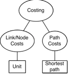
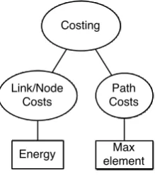
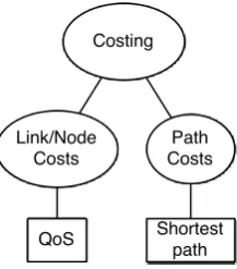
3.3 Routing protocol modules involved with the costing task . . . 41
3.4 Routing protocol modules involved with the selection task . . . 47
4.1 Typical module options for minimum hop routing protocols . . . 52
4.2 If a node is delayed in responding, the shortest path may not be returned . . 55
4.3 Typical module options for hierarchical routing protocols . . . 59
4.4 Typical module options for geographical routing protocols . . . 62
4.5 Typical module options for energy aware routing protocols . . . 65
4.6 Typical module options for routing protocols that form load balanced trees . 69
4.7 Typical module options for congestion adaptive routing protocols . . . 72
4.8 Typical module options for minimum energy routing protocols . . . 74
4.9 Typical module options for multipath routing protocols . . . 79
5.1 An example network with two sinks and seven sources. Sources B-F are
referred to as group Z for convenience . . . 90
5.2 Two example networks with and without source J . . . 101
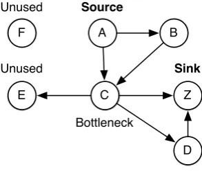
6.1 An example network showing bottlenecks and unused nodes . . . 116
6.2 The loss of node D has more impact on the network than the loss of node E 117
6.3 Node degree is not an indicator of how relied upon a node is in routing . . . 119
6.4 Two example networks with minimum and maximum clustering coefficient 120
6.5 The clustering coefficient is unusable . . . 120
6.6 Removing any intermediate node does not cause the shortest path length to
increase between any source and sink . . . 121
6.7 Being on the minimum hop path is not indicative of a node’s importance in
routing . . . 122
6.8 It is not clear which path should be selected . . . 124
6.9 An example network with two sources, A and D . . . 126
6.10 An example network with two sources, A and D . . . 127
6.11 A tree showing simple paths from sources A and D to sink Z . . . 128
6.12 An example network with two sources, A and D . . . 130
6.13 A tree showing simple (source, sink) paths from source A . . . 130
6.14 A fully connected network of 7 nodes, including 1 source and 1 sink . . . . 131
6.15 An example network showing simplest paths . . . 133
6.16 An example network with two sources, A and D . . . 134
6.17 A tree of simplest paths that is formed from an example network . . . 136
6.18 A tree of simplest paths that is formed from an example network . . . 137
6.19 Adding link AG causes simplest paths to become non-simplest . . . 138
6.20 The worst-case scenario layout for generating simplest paths . . . 141
6.21 An example network . . . 143
6.22 A contraction of the network shown in Figure 6.21 . . . 143
6.23 Multi-edge examples . . . 144
6.24 An example network with two sources (A and D) and one sink (Z) . . . 145
6.25 A tree showing simplest paths from sources A and D to sink Z . . . 145
6.26 A tree showing simplest paths from sources A and D to sink Z . . . 146
6.27 The worst-case scenario layout for generating simplest paths . . . 147
6.28 Contracting a network may allow a more accurate measurement of node
reliance values . . . 148
6.29 An example network with two sources, A and D . . . 150
7.1 Node positions for triangular, square and hexagonal node placements . . . . 158
7.2 SimpleLex CWT vs. number of simple paths . . . 169
7.3 SimplestLex CWT vs. number of simplest paths . . . 170
7.4 CWT vs. proportion of sources for networks with 10 nodes and 1 sink.
Error bars represent one standard deviation . . . 172
7.5 CWT vs. proportion of sources for networks with 20 nodes and 1 sink.
Error bars represent one standard deviation . . . 173
7.6 CWT vs. proportion of sources for networks with 40 nodes and 1 sink.
xi
7.7 MinHop route from source 9 to sink 5 . . . 175
7.8 Total data transfer vs. proportion of sources for networks with 40 nodes
and 1 sink. Error bars represent one standard deviation . . . 178
7.9 Total data transfer vs. proportion of sources for networks with 20 nodes
and 1 sink. Error bars represent one standard deviation . . . 181
7.10 Total data transfer vs. number of nodes/sources for networks with 1 sink.
Error bars represent one standard deviation . . . 183
7.11 CWT vs. number of nodes/sources for networks with 1 sink. Error bars
represent one standard deviation . . . 184
7.12 CWT vs. total data transfer for 40 node/39 source/1 sink networks and 20
node/19 source/1 sink networks . . . 186
8.1 State of the network at time 1 . . . 199
8.2 State of the network at time 2 . . . 200
8.3 State of the network at time 3 . . . 201
8.4 State of the network at time 4 . . . 202
8.5 State of the network at time 7 . . . 209
8.6 State of the network at time 8 . . . 210
8.7 State of the network at time 9 . . . 211
8.8 State of the network at time 10 . . . 212
8.9 State of the network at time 11 . . . 213
8.10 State of the network at time 15 . . . 221
8.11 State of the network at time 16 . . . 222
8.12 State of the network at time 47 . . . 223
8.13 State of the network at time 48 . . . 224
8.14 State of the network at time 0 . . . 236
8.15 State of the network at time 1 . . . 237
8.16 State of the network at time 2 . . . 238
8.17 State of the network at time 3 . . . 239
8.18 State of the network at time 4 . . . 240
8.19 State of the network at time 5 . . . 241
8.20 State of the network at time 10 . . . 242
8.21 State of the network at time 11 . . . 243
8.22 State of the network at time 12 . . . 244
8.24 State of the network at time 40 . . . 246
8.25 State of the network at time 41 . . . 247
8.26 State of the network at time 42 . . . 248
8.27 State of the network at time 43 . . . 249
8.28 State of the network at time 50 . . . 255
8.29 State of the network at time 51 . . . 256
8.30 Mean node reliance error varies with the proportion of simple paths known 257
8.31 Many simple paths may travel through a single node . . . 258
9.1 CWT vs. proportion of sources for networks with 10 nodes and 1 sink . . . 272
9.2 CWT vs. proportion of sources for networks with 20 nodes and 1 sink . . . 273
9.3 CWT vs. proportion of sources for networks with 40 nodes and 1 sink . . . 274
9.4 Total data transfer vs. proportion of sources for networks with 10 nodes
and 1 sink . . . 277
9.5 Total data transfer vs. proportion of sources for networks with 20 nodes
and 1 sink . . . 278
9.6 Total data transfer vs. proportion of sources for networks with 40 nodes
and 1 sink . . . 279
9.7 Total data transfer vs. number of nodes/sources for networks with 1 sink . . 281
9.8 CWT vs. number of nodes/sources for networks with 1 sink . . . 282
10.1 CWT vs. proportion of sources for networks with 40 nodes and 1 sink . . . 292
10.2 Total data transfer vs. proportion of sources for networks with 40 nodes
and 1 sink . . . 294
10.3 Total data transfer vs. number of nodes/sources for networks with 1 sink . . 296
10.4 CWT vs. number of nodes/sources for networks with 1 sink . . . 297
11.1 An example network split into clusters . . . 307
11.2 A representation of Figure 11.1 with a source replacing each cluster . . . . 307
11.3 A detailed representation of cluster A from Figure 11.2 . . . 308
11.4 A detailed representation of cluster C from Figure 11.2 . . . 309
11.5 A detailed representation of cluster E from Figure 11.2 . . . 310
11.6 Removing D does not help to find the minimum complementary (source,
sink) vertex cut of D . . . 312
xiii
A.1 The dashed lines indicate the region in which new nodes may be placed . . 328
A.2 Diagrams showing the formation of a triangular network . . . 331
A.3 Diagrams showing the formation of a square network . . . 332
List of Tables
2.1 Current drawn by the TMote sky in different scenarios . . . 17
5.1 Simulation of experiment 1 . . . 102
5.2 Simulation of experiment 2 . . . 102
6.1 Simple paths from sources A and D to the sink Z from the network of
Figure 6.10 . . . 127
6.2 Reliance values calculated from the simple paths shown in Table 6.1 . . . . 129
6.3 Simple and simplest paths from the network of Figure 6.16 . . . 134
6.4 Reliance values calculated from the simple paths shown in Table 6.3 . . . . 135
6.5 Relative and absolute reliance values calculated from the contracted simple
paths of Figure 6.24 . . . 146
6.6 Reliance values calculated from Figure 6.29 using the simple paths model . 150
7.1 Results of the experiment when used with static data rates. . . 163
7.2 Maximum simulation time for simulating a network of up to 20 nodes for
each heuristic . . . 164
7.3 Normalised average transmissions per message received at the sink for
net-works of 20 or fewer nodes . . . 166
7.4 Normalised average overheard messages per message received at the sink
for networks of 20 or fewer nodes . . . 166
7.5 Results of experiment when used with random data rates. . . 167
7.6 Difference of using static and random data rates . . . 167
8.1 Constant values for the enumeration algorithm examples . . . 197
8.2 Constant values for the enumeration algorithm examples . . . 233
9.1 Values of constants in the global knowledge routing protocols . . . 265
9.2 Values of constants in the enumeration routing protocols . . . 266
9.3 Values of constants in the EnergyAware routing protocol . . . 267
9.4 Values of constants in the MOR routing protocol . . . 267
9.5 Normalised CWT and total data transfer metrics for each routing protocol
with a perfect radio model . . . 269
9.6 Normalised average transmissions per message received at the sink . . . 270
10.1 Normalised CWT and transfer metrics for each routing protocol with a
real-istic radio model . . . 288
10.2 Difference between the normalised CWT and total data transfer metrics in
perfect and realistic physical models . . . 290
11.1 Reliance values for the network of Figure 11.2 . . . 308
11.2 Reliance values for the network of Figure 11.4 . . . 309
Chapter 1
Introduction
Wireless Sensor Networks (WSNs) consist of distributed, autonomousnodesthat work to-gether to observe some phenomenon of interest by taking sensor readings of factors such
as temperature, humidity and radiation. WSNs have been used for many applications,
including animal tracking [111][128][18][50], structural monitoring [122][71][17],
envir-onmental monitoring [9][114][119] and resource monitoring in offices and homes [62][53].
Data is collected in a WSN by transferring it from source nodes that generate data to sink
nodes that collect it. The nodes are battery powered and thus can only operate for a limited
period of time. Once the energy has been exhausted from a node, it ceases to function and
its loss may inhibit other nodes in the network. In many applications, data is transferred
by routing, which may consume the majority of the battery life and potentially render the
WSN unusable.
This thesis examines the problem of keeping WSNs as useful as possible for as long as
possible. It presents a new basis for routing known asnode reliance, which assigns a cost to each node based on the degree to which it is relied upon in routing data from sources to
sinks. As will be discussed in Section 1.3, in many applications, the usefulness of a WSN
at a particular instant is considered to be proportional to thesource diversityof data that it collects, where source diversity is defined as the number of sources used to provide a set of
data.
It is hypothesised that by routing using node reliance, it is possible to achieve a high source
diversity for longer than with other routing protocols.
1.1
Wireless Sensor Networks
Historically, WSNs have been characterised as wireless networks consisting of numerous
small, energy constrained, low cost, autonomous nodes that are distributed over an area for
the purpose of monitoring or sensing [48] [96] [24]. Communication or relaying of data
typically occurs via wireless multi-hop routing. The majority of WSNs exhibit a (source,
sink) architecture, which may include any number of:
1. source nodes, which generate data, usually by using sensors to measure environ-mental factors such as temperature, humidity or radiation,
2. sinknodes, which collect all data gathered by source nodes, and
3. intermediatenodes (which may include source nodes) that aid the transmission of data from sources to sinks.
The generation of data at source nodes occurs either proactively or in response to some
request. It has been suggested that sink nodes, which are often referred to as base
sta-tions, may be high powered [19], linked to databases via satellite links [96] or have more
resources than other nodes [49].
Despite the difficulties with limited energy capacities and the need to engage in multi-hop
routing in order to collect data, WSNs offer a number of advantages over conventional
environmental monitoring systems. In particular it is anticipated that WSNs will be rapid
to deploy [49], adaptable [32][69] and self configuring [15][38][11][16], thus reducing the
effort required to set up the devices and lowering costs of data gathering.
1.2
Routing Protocols
As indicated in Section 1.1, source nodes typically transmit data to sink nodes through
multi-hop routing. In this thesis, routing and dissemination are differentiated by the
fol-lowing definitions:
3
[47] in which pairs of nodes negotiate the data that will be exchanged to ensure that
only required data is transmitted.
• Routing heuristicsare a set of algorithms or procedures that perform acostingtask in which costs are assigned to available paths to indicate how desirable they are and
aselectiontask in which a path is selected.
• Routing protocolsare a set of algorithms or procedures that carry out the functionality of a routing heuristic as well as adiscoverytask in which data regarding the network is collected.
The discovery, costing and selection tasks will be discussed in further detail in Chapter 3.
The use of radio in WSN applications is known to be a heavy user of the battery, even when
receiving data [94][24][92]. Given the limited energy reserves of nodes, it is important for
dissemination protocols, routing protocols and heuristics to limit any wastage of energy
and select paths that will extend the time for which the network remains functional.
As will be shown in Chapter 4, many routing protocols will only work under ideal
condi-tions in which radio transmissions are never lost and the nodes always transmit in a
per-fectly circular shape. Furthermore, very few routing protocols avoid forming contentious
paths amongst sources, i.e. the optimal path from every source may include a common
subset of nodes. Those routing protocols that do avoid contention are often wasteful of
network resources by e.g. expending energy to avoid contention or using paths that result
in excessive battery drain on nodes. If sources do not avoid contention, it is possible that
one or more nodes may be exhausted due to overuse and the network may be partitioned.
When a partition occurs, sources are disconnected from sink nodes, thus reducing source
diversity and potentially the total data transferred from sources to sinks.
1.3
Motivation and Problem Statement
Certain applications benefit from having a high source diversity for as long as possible,
since this leads to an increased resolution of data and allows a domain expert to extract
There are several examples [111][128][81][114][71][119] in the literature of WSN
applic-ations that benefit from receiving data from a variety of sources for as long as possible.
For example, CenseMe [81] is a social-networking WSN application, designed to operate
on mobile phones, which act as source nodes. The application infers what a user is doing
(and with whom) by means of the microphone, GPS receiver, accelerometer and bluetooth
receiver. For example, the bluetooth receiver and accelerometer may allow the inference
that Alice is walking with Bob. The WSN remains functional even if individual sources
are switched off. However, as the number of concurrently operating sources increases, it
is possible to get more information from the data that is received from them. In the above
example, if Bob deactivates his source, it is only known that Alice is walking. Conversely,
if Jon switches his phone on, it becomes known that Jon, Alice and Bob are all walking
together.
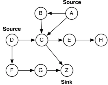
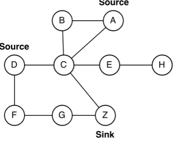
Consider the network shown in Figure 1.1. It consists of nine nodes (A-H and Z) of which
two are sources (A and D) and one is a sink (Z). An edge between two nodes indicates
that those nodes can communicate with each other. Within the network, it is obvious that
certain nodes are more important to maintaining (source, sink) connectivity than others.
For example, the loss of sink Z renders the network useless. The loss of node C makes
source A useless, but allows source D to continue operating. Finally, the loss of node E or
H has no effect.
Z
Sink
A
Source
B
C D
F G
E
Source
[image:33.595.174.356.453.596.2]H
Figure 1.1: An example network with with 9 nodes, including 1 sink and 2 sources
The problem is to find a routing protocol that will create as great a source diversity for as
long as possible, i.e. it will keep as many sources connected to sinks for as long as possible.
In most routing heuristics, each source determines the optimal path for routing to a sink.
5
source D. However, both of these routes require the use of node C, a node that is essential
for the operation of source A.
A cooperative scheme may require source D to use the non-optimal route DFGZ, thus
reducing the energy expenditure of node C and allowing both sources to remain connected
simultaneously for longer.
1.4
Assumptions
The following assumptions are made for the purpose of this thesis:
• Battery drain from computation is negligible compared to that from radio.
• Communication in the network may be imperfect.
• Nodes are immobile.
• The energy on each node is limited and cannot be replenished. These assumptions will be examined in further detail in Chapter 2.
1.5
Approach: Node Reliance
This thesis presents a new family of routing heuristics known asnode reliance, which aim to maintain a high source diversity for as long as possible, i.e. to keep sources connected
to sinks. The node reliance heuristics are later extended into routing protocols for use in
WSNs.
The premise of node reliance routing is that each node is assigned a weighting, which gives
an indication of how much that node is relied upon in routing from sources to sinks. The
routing protocol will preferentially avoid using routes containing nodes of high reliance.
Node reliance acts cooperatively in that sources determine routes based on a holistic view
It is hypothesised that by routing using node reliance, it is possible to achieve a high source
diversity for longer than with other routing protocols.
1.6
Contributions
This thesis makes four original contributions:
• A modularised view of routing protocols,
• A family of new routing heuristics and routing protocols namednode reliance,
• A new metric named Connectivity Weighted Transfer (CWT) that may be used to measure source diversity over time, and,
• An experimental analysis of routing heuristics and protocols and their suitability in different operating conditions to maintaining source diversity.
The modularised view of routing protocols demonstrates the way in which the behaviour
of many routing protocols can be separated into a number of differentmoduleseach with different objectives, features, advantages and disadvantages. Using such a view makes it
possible to compare routing protocols and to construct new ones to meet particular
applic-ation features by assembling modules.
Node reliance is the new family of routing heuristics and routing protocols that aim to
maintain source diversity for as long as possible in a WSN.
CWT is a new metric that is introduced in order to measure source diversity over time.
Source diversity relies on connectivity between sources and sinks. A common measure
of connectivity is the total number of bytes transferred from sources to sinks. However,
this measurement does not distinguish whether the data is received from a single source or
whether it comes from many sources, the latter of which is preferred. CWT measures the
total data transferred, but the score is biased. A user-definedweighting factorcan be used to indicate whether it is preferable to have:
7
• few sources connected for a long time.
The ability to bias numerous connections over a possibly shorter period of time is
import-ant, since this thesis is interested in maintaining source diversity for as long as possible.
Finally, an experimental analysis of routing heuristics and routing protocols, including the
node reliance family and third party approaches is carried out. Measurements include both
CWT and the more commonly used total data transfer in order to establish under which
conditions each routing protocol is able to best obtain source diversity for as long as
pos-sible.
1.7
Thesis Structure
The thesis is structured as follows:
Chapter 2 discusses WSNs and justifies the assumptions made in this thesis regarding their
capabilities and restrictions. Chapter 3 presents the modularised view of routing
proto-cols. Related work, including common routing protocol paradigms and their suitability to
the problem solution are discussed in Chapter 4. Chapter 5 deals with measuring source
diversity in WSNs. Specifically, this chapter covers different metrics, including the new
CWT metric as well as an experimental methodology for measuring the source diversity
provided by using different routing protocols. The new node reliance heuristics are
pro-posed in Chapter 6 and analysed in Chapter 7. The node reliance routing protocols are
proposed in Chapter 8. The routing protocols are analysed under perfect conditions in
Chapter 9 and under realistic conditions in Chapter 10. Finally, conclusions and further
Chapter 2
Wireless Sensor Networks
This chapter examines the characteristics of WSNs and justifies the assumptions made
in Chapter 1. The literature is inconsistent regarding the capabilities and characteristics
of WSNs. Often, the description or assumptions of the system are unspecified. These
problems make it difficult to analyse a WSN system and find solutions to many of the
problems they face. In this chapter, several assumed WSN characteristics from the literature
are analysed in order to develop a definition of WSNs that will be used consistently in the
remainder of the thesis.
2.1
Overview
Historically, WSNs have been characterised as wireless networks consisting of numerous
small, energy constrained, low cost, autonomous nodes that are distributed over an area for
the purpose of monitoring or sensing [48] [96] [24]. Communication or relaying of data
typically occurs via wireless multi-hop routing. The majority of WSNs described in the
literature exhibit a (source, sink) architecture, which may include any number of:
1. source nodes, which generate data, usually by using sensors to measure environ-mental factors such as temperature, humidity or radiation,
2. sinknodes, which collect the data gathered by source nodes, and
3. intermediatenodes, which may include source nodes, that aid the transmission from sources to sinks.
The generation of data at source nodes may occur either proactively or in response to some
request. It has been suggested that sink nodes, which are often referred to as base
sta-tions, may be high powered [19], linked to databases via satellite links [96] or have more
resources than other nodes [49].
WSN nodes are typically battery powered and for reasons expounded upon in Section 2.5.4,
the energy of a node is used to refer to its remaining battery power within this thesis. The
energy capacity of a battery is dependent on its size and since nodes are expected to be
small, the batteries are unlikely to be of high capacity. It has been suggested [33] that
battery depletion is one of the key challenges experienced in developing and working with
WSNs, particularly since every operation performed by the node requires expenditure of
energy [31]. While other resources such as the CPU, memory or storage may be
immedi-ately re-used when released, the same is not true of the battery. Unless a node has some
means of energy replenishment, which is discussed in Section 2.5.4, the capacity of
batter-ies restricts both the maximum lifetime of nodes and the frequency with which the node
can carry out particular actions.
Beyond these characteristics, it is difficult to provide a formal definition of the exact
cap-abilities of a WSN, particularly due to the increasing number of scenarios making use of
the technology [96]. It has been theorised that, with WSNs typically being application
dependent, it will never be possible to create a single architecture, which can be used in
all applications [59]. Without a single architecture being defined, it may be impossible to
precisely define the characteristics of a WSN. R¨omer has created a design space [96] that
discusses the large number of dimensions in WSN deployments, including:
• deployment type,
• node mobility,
• node size,
• node cost (in dollars),
11
• heterogeneity of nodes,
• method of wireless communication,
• infrastructure,
• network topology,
• sensor coverage,
• connectivity,
• number of nodes,
• estimated running time, and,
• quality of service.
Most of these categories are self-explanatory. Thedeployment typerefers to the method by which nodes are physically deployed, i.e. whether nodes are deployedone timeor whether they areiteratively replenished and whether their placement is randomormanual. Infra-structure specifies how routing occurs within the network; possible values are ad hoc in which nodes may communicate with each other andbase stationin which nodes may only directly communicate with a base station. Thenetwork topologyaffects how nodes are in-terconnected, i.e. which nodes may communicate with each other.Sensor coveragereflects the density of source nodes, i.e.sparseordense. In an extreme case, the sensor coverage may beredundantso that multiple sources cover the same area. Theconnectivityof a net-work indicates the frequency with which any two nodes may communicate. For example
there is always a path between any pair of nodes in a connectednetwork. In an intermit-tentnetwork, pairs of nodes may be occasionally partitioned. Finally, if nodes are usually isolated but occasionally come into contact with each other then the network is said to have
sporadicconnectivity.Quality of servicerequirements include any constraints that may be placed on the network. Examples include the requirement that data must be received by
a sink within some period of it being generated by a source, and that the network must
remain operational with a certain degree of node loss.
The survey carried out by R¨omer shows that the majority of deployments considered
in-volve tens of battery-powered nodes that are manually placed and communicate via radio.
2.2
Relationship to Wireless Ad Hoc Networks
R¨omer’s design space [96] indicates that the infrastructure of certain WSNs may be ad hoc,
i.e. nodes may freely communicate and route through each other. Since communication
in a WSN also takes place wirelessly, the field of Wireless Ad hoc Networksmay contain relevant literature to the field of WSNs. In particular, research involving wireless
com-munication, routing and resource management is of interest to both fields and so may be
relevant to either domain.
Even though the literature does not consistently attribute any other features to wireless ad
hoc networks, it has been suggested [120][98] that there are substantial differences between
WSNs and ad hoc networks. For example, Royer [98] suggests that WSNs are deployed
for a specific task, whereas wireless ad hoc networks are a result of mobile users joining
a stationary network using mobile devices such as phones. However, such a distinction is
inadequate, since nodes in a WSN may be dynamically reprogrammed [32], thus changing
the task for which they were deployed. Furthermore, if sources are mobile and sinks are
static, then a WSN may consist of a stationary network in which mobile nodes join and
leave the network. Such behaviour is also covered in R¨omer’s design space, in which
connectivity may be sporadic, sources may be mobile and sink nodes may be static.
In the literature, there are many examples of work that was designed for wireless ad hoc
networks and is readily referenced in work on WSNs. For example, AODV [89] was
ini-tially designed for a wireless ad hoc network and yet is commonly referenced and used as
a basis for comparison in work on WSN routing protocols [12] [103] [106] [79] [117] [10].
Similarly, the GPSR [60] or DSR [54] routing protocols, frequently referenced in the WSN
literature, were initially designed for wireless ad hoc networks.
Due to the overlap of these areas, research that is aimed at wireless ad hoc networks is
included alongside work on WSNs.
2.3
Advantages
Traditionally, environmental monitoring would be carried out using networks of wired
13
cameras and microphones [18]. WSNs offer a number of advantages over these systems,
such as being:
• self configuring and adaptable, [18],
• quickly deployable [49],
• low cost [49][8], and
• usable in inhospitable areas [33].
These advantages are described in more detail below.
WSN nodes are envisioned as being able to configure themselves [49] in order to
sat-isfy application goals. Once nodes are deployed, routes from sources to sinks are
auto-matically found and used. Source nodes whose sensing areas overlap can schedule the
times at which they are active to minimise data duplication and maximise operational time
[15][38][11][16]. Adaptability allows the network to respond to the expiration of nodes
as well as to make use of new nodes that are added to the network [49]. A user may also
adjust the behaviour of a WSN. For example, the user may be able to control what data the
network collects. In an extreme case, users can dynamically reprogram nodes to change
the way in which they operate [32][69].
WSNs are fast to deploy, since nodes are self-configuring and need not be wired together
[49]. Furthermore, since a WSN can adapt to the addition of nodes, it is possible for a
network to be incrementally deployed at the convenience of the operator [49].
It has been suggested that, since nodes are small and individually have little processing
power, as the number of manufactured nodes increases, the cost of nodes will drop perhaps
to less than a dollar each [49][8]. Costs can also be reduced by the lack of wiring required
to connect nodes and by the improved deployment time, which can reduce money spent on
human effort.
The final advantage of a WSN over traditional systems is the ability to deploy the system
in an inhospitable environment. Since a WSN is potentially adaptable and self-configuring,
there is no need for prolonged human intervention in running the network. It may therefore
2.4
Example Deployments
In order to give examples of WSN usage, this section discusses a number of deployments
that feature prominently in the literature. For each deployment, details of the number of
nodes that constitute the deployment, a summary of the data collection mechanism, and the
WSN’s resilience to source loss, which reflects how the expiration of sources affects the
system, are provided. These features can be used to express the data collection behaviour
of an application and so can be used to summarise how the deployment works and under
what conditions it remains useful.
Since many proposed WSN applications have been shown to be impractical or unfeasible
[112], only those applications that have been physically deployed or deployed in a test
environment are considered. Applications that have only been proposed or theorised are
not discussed.
One of the best-known WSN deployments is the habitat monitoring of Great Duck Island
(GDI) [111]. 150 source nodes were placed on the island. Two types of source were used:
burrow nodes to monitor the nesting burrows and weather nodes to measure the ambient
weather conditions of the island. The application did not require all sources to be alive and
nodes expired at various times throughout the 120-day deployment.
ZebraNET [128] used a WSN to track the locations of zebras in Kenya. The deployment
of nodes called for 30 specially built collars to be attached to zebras. Each collar acted as
a source node and contained solar panels, a small battery, a radio and a GPS receiver. GPS
data was periodically gathered and stored at each source. Unlike many other deployments,
ZebraNET used a dissemination protocol in which any data collected by a source was distributed to all other sources in the network. Since the application gathered the positional
data of each zebra, it remained operational even if some source nodes expired. However,
the number of correlations between zebra positions would be reduced.
Wisden [122] is a system for structural monitoring in which source nodes are manually
placed on a structure, such as a bridge, to monitor vibration levels using sample rates of
around 100 Hz. All data is stored at source nodes and periods of interesting activity i.e.
consecutive data samples that differ and lie above some threshold, are forwarded to a sink.
The authors note that Wisden is intolerant to data loss and consequently all sources must
15
CenseMe [81] is a social-networking WSN application, which is designed to operate on
mobile phones (specifically, the Nokia N95). The application takes periodic readings from
the accelerometer, microphone and GPS receiver. It also takes periodic random photos
using the built-in camera and uses the Bluetooth receiver to detect other nearby CenseMe
users. Combining all of this information, the application attempts to infer what the user is
currently doing. For example, by using the microphone, the application may determine that
the user is engaged in conversation. Similarly, the accelerometer may determine whether
the user is standing, sitting, walking or running. In the application’s test deployment, 22
people ran the CenseMe application as they went about their daily lives. Since users could
simply switch their phones off at any time, it is concluded that CenseMe is capable of
operating with source loss, albeit with reduced functionality.
A system for analysing the microclimates surrounding redwood trees has been produced by
Tolle [114]. In Tolle’s deployment, 33 source nodes were placed approximately 2m apart
on a single tree between 15 metres and 70 metres off the ground. Each source generated and
stored periodic data based on temperature, humidity and radiation readings before routing
it to a sink at the bottom of the tree. The author notes that analysis remains possible with
source loss and so hence, not all sources are required for the application to be functional.
NAWMS [62] provides fine granularity detail regarding water usage in homes. By placing a
source node on each water pipe and a sink node at the water meter (an accurate device that
measures water flow through the entire building), NAWMS can calibrate pipe vibrations
against water flow. Once the system is calibrated, it provides real-time data regarding
water usage for each device. It is estimated that a house with 3 bedrooms and 2 bathrooms
may require between 17 and 21 sources. For such a system to be correctly calibrated, every
source would have to be operational. If individual sources failed then the water meter’s
measurement would not correspond with the monitored vibration of the pipes. Thus the
loss of any source would appear to render the system unusable.
PermaSense [9] aims to gather environmental data regarding permafrost in the Alps for at
least 3 years. Approximately 25 sources form a wireless network in which environmental
data is periodically gathered, stored and routed to a sink. The project has tight constraints
regarding the loss of data; specifically, 99% of data must be recovered and no more than
10 consecutive points of data may be lost. Consequently, the loss of even a single source
SASA [71] (the structure-aware self-adaptive WSN system) is an application to monitor
the structural integrity of mines. One particular test deployment used 27 source nodes
and a single sink to monitor a tunnel. Sources were mounted to the walls, ceiling and
floor. Each source monitored its neighbours (i.e. the closest six sources) by the periodic
exchange ofbeacons. If, during some time period T, two of a source’s neighbours were to change, the network would infer that a collapse had taken place and send a report to the
sink. Each source was pre-programmed with its location in the tunnel, and consequently it
was possible to determine the size and location of any hole that was formed. SASA has a
limited resilience to source loss. If too many sources are lost in one area or in a short space
of time, the ability to detect collapses may be compromised.
Werner-Allen has used WSNs for monitoring the Reventador volcano in Ecuador [119].
16 source nodes used seismometers and microphones sampling at 100 Hz to carry out
measurements. If a source detected a seismic event, it would forward its readings to the
sink. The sink then queried other sources for readings during that time period to gain a
complete view of all sources during possible seismic events. A small number of sources
were lost during the operation of the network, leading to the conclusion that the application
remains operational with source node loss.
Ceriotti has deployed a WSN to monitor the health and deformation of the medieval Torre
Aquila tower located in Trento, Italy [17]. The deployment consisted of 16 sources, plus a
sink node. Sources measured either deformation of the structure, vibrations or temperature
and forwarded readings towards the sink every period of time. Several forms of analysis
were carried out such as structural deformation versus temperature. It was therefore
ne-cessary for certain numbers of each type of source node to remain active in order for all
analysis to be carried out.
2.5
Assumptions
In Section 1.4, the following assumptions are made for the purpose of this thesis:
• Battery drain from computation is negligible compared to that from radio.
17
Table 2.1: Current drawn by the TMote sky in different scenarios
Activity Nominal Current (mA)
Radio receiving, MCUaon 21.8
Radio transmitting, MCU on 19.5
Radio off, MCU on 1.8
Radio off, MCU idle 0.0545
Radio off, MCU standby (low power) 0.0051
aAlthough not defined in the document, it is believed that MCU refers to
the micro controller unit, i.e. the processor.
• Nodes are immobile.
• The energy on each node is limited and cannot be replenished. These assumptions are justified in the following sections.
2.5.1
Battery Drain from Computation
This thesis assumes that the battery drain from carrying out computation is negligible when
compared to that caused by usage of the radio.
A radio can be a major cause of battery depletion in nodes [94], whether it is transmitting
or receiving [92]. The TMote sky [101] is a recent, generic, commercially available WSN
platform. Table 2.1 shows how much current is drawn by the TMote sky in particular
scenarios according to the TMote sky data sheet [101].
The table reveals two interesting facts.
Firstly, it shows that using the radio to receive and transmit draws a large current but also
that the current drawn for receiving is more than the current drawn for transmitting. Thus,
it is unreasonable to disregard energy expenditure in receiving transmissions.
Secondly, even if the radio’s usage of the processor is disregarded (21.8 - 1.8 = 20 mA for
the radio alone), the current used when receiving data on the radio is 11.1 times higher than
the current used by the processor (1.8 mA). These figures also assume that the processor
it would when sampling from a sensor and then forwarding the result to the radio, then the
processor will be mostly idle. Thus, the current used when receiving data on the radio may
be 3922 times higher than that used by the idle processor (0.0545 mA). If the processor
enters a low power mode rather than merely remaining idle, the current would be expected
to be even lower.
These numbers suggest that the battery depletion due to radio use is significantly higher
than that of using the processor. Given that the onboard processor of nodes is relatively
slow, it is more likely that a complex computation will be impractical by reason of its long
running time rather than the energy it is likely to use. It is therefore reasonable to assume
that the depletion of the battery caused by computation is negligible when compared to the
depletion caused by using the radio.
2.5.2
Imperfect Communication
In a WSN, nodes communicate with each other wirelessly and usually via low powered
radio. The use of wireless communication has a number of distinct challenges or features
that are not present or less problematic in wired communication.
Firstly, communication between a pair of nodes may be unreliable, i.e. packets may be
lost. Secondly, communication may be unidirectional, i.e. node A can transmit to node B,
but node B cannot transmit to node A. These problems are discussed in more detail in the
following sections.
2.5.2.1 Unreliability
Wireless communication is unreliable and there is always a small probability that a packet
will be lost [109]. In this section, the cause of the unreliability and its immediate
con-sequences are discussed.
In wireless communication, a radio signal is transmitted with a certain power. As the signal
travels through the air, it attenuates (degrades) and may be absorbed by particles in the air,
physical obstacles and the ground. For a low-lying antenna that transmits a signal across a
19
distance travelled [92] [14]. For example, a signal that travels a distancedwill degrade by
a factor ofd4. If the distance is doubled, the signal’s quality will decline by 16 times (24).
It is often assumed that the relationship between the transmission power and distance isd2
rather thand4 [46]. In either case, transmitting a signal across a bigger distance will cause
a bigger degradation of the signal and so transmissions must be made with high power to
ensure they are received. WSNs that are deployed over large areas must therefore either use
very large amounts of energy or must engage in multi-hop routing in order to communicate.
The probability that a node A receives a transmission from B is proportional to the
dif-ference between the received signal strength of B’s transmission at A and the sensitivity
of A’s radio. If the sensitivity of A’s radio is exactly equal to the signal strength then the
transmission is lost with probability 1. Signal strength is affected by the power with which
the transmission is made, the attenuation of the signal, background noise and interference
from other radio transmissions. The latter two factors are random, and thus there always
remains a small probability that a transmission may be lost.
Complicating the problem is the fact that although attenuation is approximately
propor-tional to the 2nd or 4th power of distance, it is not uniform.
If it is known that a packet has been lost, it is possible to transmit it again. However,
confirming packet reception at each hop may increase the number of transmissions being
made by nodes and thus drain batteries more quickly. Furthermore, in order to receive
confirmation that a packet has been received, the links between nodes must be bidirectional,
which may not be the case as will be discussed in Section 2.5.2.2.
It has been suggested that routing along paths of high stability may lower energy
consump-tion [39][40][120] since fewer retransmissions might take place. However, it is debatable
whether stable links are better formed using paths of few hops or many hops.
Woo [120] suggests that paths of many reliable links are better than paths of few unreliable
links. Paths with few hops result in nodes that are geographically distant. Since attenuation
is dependent on distance between nodes, paths with few hops are likely to involve links that
are unreliable and may have to be retransmitted, expending additional energy. If nodes are
geographically close then the transmission energies of nodes may be vastly reduced since
there is no reason for them to transmit such great distances. However, such a reduction
received.
Conversely, Haenggi [39] [40] has suggested that long hops formed as a result of an
in-creased transmission power have a higher signal to interference and noise ratio and so are
more likely to be received. Haenggi also observes that paths of fewer nodes mean that there
are fewer places in which a path can fail.
In conclusion, it should not be assumed that wireless communication is always successful.
It also remains unclear whether paths with geographically distant nodes are more or less
reliable than paths with numerous nodes that are close together.
2.5.2.2 Unidirectional Links
Wireless communication is not necessarily bidirectional. If a node A can send a message
to a node B, there is no guarantee that node B can transmit to node A. Unidirectional
links may occur because one node is capable of sending a higher energy transmission. It
may also be the case that the geographical location of the nodes makes communication
unidirectional. For example, nodes on a hill may be able to transmit to nodes in a valley,
but not vice-versa. Nodes may achieve bidirectionality by performing a limited local flood,
i.e. using other neighbouring nodes to transmit from node B to node A. However, there is
no guarantee that such a path would exist and energy would be drained as a result of trying
to find or use such a path.
One way to encourage bidirectional links is to place nodes close together, so that the
prob-ability of successful transmission is high in both directions. However, distributing nodes in
this manner will result in a highly dense network, which may not be suitable for many
ap-plications. For example, more nodes will be required to cover the same area, thus increasing
the cost of the network and potentially increasing scalability problems. Each node will also
be in transmission range of more nodes, thus increasing the number of messages received
and overheard and therefore causing its energy reserves to be depleted more quickly.
In conclusion, it is impractical to assume that links between nodes are bidirectional, since
doing so limits the networks in which an application can operate. Even if it is possible
to discard unidirectional links, the application’s efficacy may drop as a result of not fully
utilising all links in the network. In a worst-case scenario, the network may be treated as
21
2.5.3
Mobility
This thesis assumes that nodes are immobile for two reasons:
1. The majority of networks use immobile nodes.
2. If mobile nodes were permitted, the problem of keeping sources connected to sinks
becomes significantly harder to solve.
These reasons are explained in more detail below.
The majority of deployments studied in Section 2.4 use stationary nodes. The two major
exceptions are ZebraNET [128] and CenseMe [81], in which nodes are attached to animals
or people and can therefore freely move around. SASA [71] detects structural changes
in mining shafts by the sudden change in position of nodes. However, the nodes are not
considered to be mobile since many nodes change position once, simultaneously. Thus,
the change in node positions is more like a reconfiguration of the network topology than a
node position being under constant change.
The second reason for assuming immobility of nodes is that there may be no universal
solution to maintaining high source diversity for long periods of time if the topology is
consistently changing. Since the movement of nodes may be random, the importance of any
node may change at any time. Nodes that were vital may become irrelevant and irrelevant
nodes may become essential to routing. The connectivity of the network is therefore based
on a largely random factor and the success of any approach at maintaining (source, sink)
connectivity over time is dependent on that random movement.
2.5.4
Scavenging and Replenishment
It is assumed that replenishment of batteries by scavenging energy from the environment
is not possible. Although several approaches have been suggested for energy scavenging,
such as via solar cells [31][56] or nearby vibrations [97] there are two limitations, which
greatly restrict the scenarios in which scavenging can take place:
2. Nodes are restricted as to when they may expend energy.
These restrictions are summarised below.
Firstly, scavenging can only take place when there is some source of plentiful energy
avail-able. For example, if nodes are placed within buildings, pockets or away from direct
sun-light, e.g. a forest, the nodes may be unable to gather sufficient energy for the applications
to operate. Even indoor lighting may be insufficient, since it produces 2500 times less
energy than can be achieved with direct sunlight [97]. Similarly, many applications would
require a reliable, consistent and nearby source of vibrations in order to operate, which may
not be available. A further problem is that the amount of energy that can be scavenged is
dependent on the size of the node, with bigger nodes scavenging more energy [97].
How-ever, as stated in Section 2.1, WSN nodes are generally perceived as being small. Thus, the
amount of energy that can be scavenged is also likely to be limited.
Secondly, nodes will be greatly restricted in their ability to expend energy. For example
if a node relies on scavenged energy, such as solar power, it may be unable to respond to
events of interest early in the morning when its energy levels are low. Similarly, if several
cloudy days pass then the node may be unable to recharge its energy supply and the node
may be forced in to a low power mode until the sun comes out. Thus, the environment that
supplies the energy restricts the operation of the network.
These limitations do not rule out the possibility of energy scavenging. However, there are
clearly many applications where it is not appropriate and thus our assumption that energy
scavenging is not present is reasonable.
Since a node’s energy is limited to its battery power, this thesis uses the term energy to refer to energy that is provided by the battery.
2.6
Summary
This chapter presents a definition of WSNs and justifies the assumptions that are presented
in Chapter 1. It is argued that WSNs consist of numerous autonomous immobile nodes
of finite battery power. Source nodes use onboard sensors to sense or monitor the local
23
through intermediate nodes (that might include other sources) towards a sink node which
may be mains powered or may have more capabilities than other nodes in the network such
as satellite links or more powerful processing capabilities.
This chapter provides a basis on which to discuss WSNs. Having justified their capabilities
and limitations; it is possible to find a solution to the problem of routing to achieve high
source diversity for long periods of time. Chapter 3 presents a new modularised view of
routing protocols, which is used in Chapter 4 to compare different routing protocols in the
literature and their ability to solve the problem of maintaining source diversity for as long