Constructing constrained version of magic squares using selection hyper heuristics

Constructing Constrained-Version of

Magic Squares Using Selection

Hyper-heuristics

Ahmed Kheiri and Ender ¨

Ozcan

University of Nottingham, School of Computer Science Jubilee Campus, Wollaton Road, Nottingham, NG8 1BB, UK

Email: {axk,exo}@cs.nott.ac.uk

A square matrix of distinct numbers in which every row, column and both diagonals has the same total is referred to as a magic square. Constructing a magic square of a given order is considered as a difficult computational problem, particularly when additional constraints are imposed. Hyper-heuristics are emerging high level search methodologies that explore the space of heuristics for solving a given problem. In this study, we present a range of effective selection hyper-heuristics mixing perturbative low level heuristics for constructing the constrained version of magic squares. The results show that selection hyper-heuristics, even the non-learning ones deliver an outstanding performance, beating

the best known heuristic solution on average.

Keywords: Magic Square; Hyper-heuristic; Late Acceptance; Computational Design Received 09 April 2013; revised 00 Month 2009

1. INTRODUCTION

Hyper-heuristics are search methodologies which build or select heuristics automatically to solve a range of hard computational problems [1, 2, 3, 4]. Selection hyper-heuristics, which were initially defined as ”heuristics to choose heuristics” in [5], are used in this study. The idea of mixing existing heuristics (neighbourhood structures) during the search process in order to exploit their strengths dates back to the 1960s [6]. Selection hyper-heuristics have been successfully applied to many different problems ranging from timetabling [7] to vehicle routing [8].

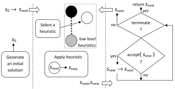
There are different types of single point-based search selection hyper-heuristic frameworks [9]. Still, two common consecutive stages can be identified in almost all such hyper-heuristics: heuristic selection and move acceptance. An initial solution is iteratively improved passing through these stages. After a heuristic is selected, it is applied to the candidate solution producing a new solution at each step. Then a move acceptance method decides whether to accept or reject the new solution. This whole process repeats until some termination criteria are satisfied as illustrated in Figure 1. [10] showed that different combinations of selection hyper-heuristic components yield different performances on examination timetabling problem.

A square matrix of distinct positive integers in which every row, column and diagonal has the same

sum is called a magic square. The history of magic squares dates back to 2200 B.C. (see [11] for more). Constructing a magic square is a computationally demanding task. Constraint version of the magic squares problem was the subject of a recent competition with the goal of finding the quickest approach. The winner approach emerged among hundreds of competing algorithms as a hill climbing algorithm [12] which handles a given instance in two separate ways based on its size. The approach mixes two heuristics with a certain probability for problems larger than a certain size and uses a different algorithm for smaller instances. In this study, we extend the framework of the winning approach to enable the use of selection hyper-heuristics for any given constraint version of the magic square problem. We investigate into the performance of a variety of selection hyper-heuristics, including the best known hyper-heuristic managing the same set of low level heuristics for constructing magic squares. Then the best selection hyper-heuristic is compared to the winning approach.

Section 2 provides the description of the magic square problem and overviews the late acceptance hill-climbing algorithm and selection hyper-heuristics. Section 3 describes the selection hyper-heuristic components that are tested for solving the magic square problem. Section 4 provides the empirical results. Finally, Section 5 presents the conclusions.

Select a heuristic

Apply heuristic Generate

an initial solution

s0→ snext

snext snew _snew → _snext

snext,snew

s0

accept( snew) ?

snext

low level

heuristics

terminate ?

return snext

yes

no no

yes

FIGURE 1. Illustration of how a single point based selection hyper-heuristic operates.

2. BACKGROUND

2.1. Magic Square Problem

A magic square of order n is a square matrix of size

nxn, containing each of the numbers 1 to n2 exactly once, in which then numbers in all columns, all rows, and both diagonals add up to the magic numberM(n). This constant is given by:

M(n) =n(n2+ 1)/2 (1) As an example, the magic square of order 3 is shown below:



43 95 27

8 1 6

 

A formal formulation of the magic square problem is as follows. Given a magic square matrix A of order n

such that

An×n=     

a1,1 a1,2 · · · a1,n

a2,1 a2,2 · · · a2,n ..

. ... . .. ...

an,1 an,2 · · · an,n     

whereai,j∈ {1,2, ..., n2}for 1≤i, j≤nandai,j ̸=ap,q for alli̸=pandj̸=q

subject to n ∑

i=1

ai,j=M(n), n ∑

j=1

ai,j=M(n), n

∑

i=1

ai,(n+1−i)=M(n) and n ∑

i=1

ai,i=M(n) Constructing the magic square using the modern heuristics was the idea of the competition hosted by SolveIT Software1_{. A constraint version of the magic}

1_{http://www.solveitsoftware.com/competition.jsp}

squares problem is used in the competition which requires for a given instance of size n ≥ 10 that the solution matrix must have a contiguous sub-matrix

S3_×3 to be placed at a given location (i, j) inAn_×n:

S3_×3=



14 25 36

7 8 9

 

The largest magic square that an algorithm constructs in one minute was considered to be the best algorithm. This was the performance measure used to determine the winner approach.

The objective (cost) function measures the sum of absolute values of the distance from the Magic number for each column, row and diagonal. Hence, the problem can be formulated to a minimisation problem in which the goal is to minimisethe objective function value in Equation 2. The magic square is found if the objective function value is 0.

g(An×n) = n ∑

i=1

n ∑

j=1

ai,j−M(n) +

n ∑

j=1

n ∑

i=1

ai,j−M(n)

+

n ∑

i=1

ai,(n+1−i)−M(n)

+

n ∑

i=1

ai,i−M(n)

(2) Equation 3 describes the objective function value after imposing the contiguous sub-matrix S3×3.

f(An_×n, i, j) =   

g(An×n) ifS3×3 placed at the position (i, j) in A;

∞ otherwise.

square is transformed into the magic square by the iterative heuristic improvement of rows and columns. Chu’s solver ranked the second on the competition and it was able to construct the constrained version of 1000x1000 magic square in one minute. The multi-step iterative local search took the third place on the competition. It was developed by Xiao-Feng Xie and it was able to construct the constrained version of 400x400 magic square in one minute. The detailed descriptions of the top three solvers are available online

at_{http://www.cs.nott.ac.uk/~yxb/IOC/}.

2.2. Late Acceptance Hill-Climbing Approach

The Late Acceptance Hill-Climbing was introduced recently, in 2008, as a metaheuristic strategy [13]. The approach has been successfully applied to many different hard-computational problems, including exam timetabling [13, 7], course timetabling [14], travelling salesman, constructing magic squares [12] and lock scheduling [15]. Most of the hill climbing approaches modify the current solution and guarantee an equal quality or improved new solution at a given step. The Late Acceptance Hill-Climbing guarantees an equal quality or improved new solution with respect to a solution which was obtained fixed number of steps before.

Algorithm 1 provides the pseudocode of Late Acceptance Hill-Climbing assuming a minimisation problem. Late Acceptance Hill-Climbing requires implementation of a queue of size L which maintains the history of solution/objective function values of L

consecutive visited states for a given problem. At each iteration, algorithm inserts the solution into the beginning of the array and removes the last solution from the end. The size of the queue L is the only parameter of the approach which reflects the simplicity of the strategy.

2.3. Related Work

Selection hyper-heuristics explore the space of heuris-tics during search process. They are high level method-ologies that are capable of selecting and applying an appropriate heuristic given a set of low-level heuristics for a problem instance [1]. A selection hyper-heuristic based on a single point search framework attempts to improve a randomly created solution iteratively by pass-ing it through firstly heuristic selection and then move acceptance processes at each step as illustrated in Fig-ure 1 [9]. The heuristic selection method is in charge of choosing an appropriate heuristic from a set of low level heuristics at a given time. The chosen heuristic is applied to a candidate solution producing a new one, which is then either accepted or rejected by the move acceptance method.

The selection hyper-heuristic framework used in this study assumes perturbative low level heuristics which

Algorithm 1Pseudo-code of the Late Acceptance Hill-Climbing (LAHC).

1: procedure_LAHC

2: S=Sinitial; ◃ Generate random solution

3: f0←Evaluate(S); ◃ Calculate initial objective function value

4: fori←0, L−1 do

5: f(i)←f0;

6: end for

7: i←0;

8: repeat

9: S′; ◃Generate candidate solution

10: f′←Evaluate(S′); ◃Calculate objective function value

11: c←imodL;

12: if f′ ≤f(c)then

13: S←S′;

14: end if

15: f(c)←Evaluate(S); ◃ Include objective value in the list

16: i←i+ 1;

17: until(termination criteria are satisfied);

18: end procedure

deal with complete solutions, as opposed to constructive heuristics which process partial solutions. [5] describe different selection methods, including Simple Random

(SR) randomly selects a low level heuristic; Random Descent (RD) randomly chooses a low level heuristic and applies it to the solution in hand repeatedly until there is no further improvement. Random P ermutation (RP) generates a permutation of low level heuristics, randomly, and applies a low level heuristic in the provided order sequentially. Random P ermutation Descent(RPD) same as RP, but proceeds in the same manner as RD. The Greedy (GR) allows all low level heuristics to process a given candidate solution and chooses the one which generates the largest improvement.

Selection hyper-heuristics could learn from their previous experiences by getting feedback during the search process. For example, [5] use a learning mechanism Choise F unction (CF) that scores low level heuristics based on their individual and pair-wise performances. [16] uses Reinforcement Learning (RL) to select from low level heuristics. [17] describe a dominance based heuristic selection method which aims to reduce the set of low level heuristics based on the trade-off between the number of steps has taken by a heuristic and the quality of solution generated during these iterative steps. The authors report that this is one of the most successful selection hyper-heuristics across multiple problem domains. Tabu [18] ranks the heuristics to determine which heuristic will be selected to apply to the current solution, while the tabu list holds the heuristics that should be avoided.

There is a variety of simple and elaborate determin-istic and non-determindetermin-istic acceptance methods used as a move acceptance component within selection hyper-heuristics. For example, accepting all moves and some other simple deterministic acceptance methods are de-scribed in [5]. There are a number ofdeterministicand

non-deterministicacceptance methods allowing the ac-ceptance of worsening solutions. The non-deterministic

na¨ıve move acceptance accepts a worsening solution with a certain probability [19]. [7] useLate Acceptance

[13], which maintains the history of objective values of previously visited solutions in a list of a given size and decides to accept a worsening solution by comparing the objective value to the oldest item in that list. [10] re-ported the success of the Simulated Annealing move acceptance method. Simulated annealing accepts non-improving moves with a probability provided in Equa-tion 4.

pt=e − ∆f

∆F(1−t

T) (4)

where ∆f is the quality change at step t, T is the maximum number of steps, ∆F is an expected range for the maximum quality change in a solution after applying a heuristic.

[20] used the Greate Deluge as a move acceptance strategy. It accepts non-improving moves if the objective value of the solution is better or equal to an expected objective value, named as level at each step. The objective value of the first generated candidate solution is used as the initial level and the level is updated at a linear rate towards a final objective value as shown in Equation 5.

τt=f0+ ∆f×(1−

t

T) (5)

whereτtis the threshold level at steptin a minimisation problem,T is the maximum number of steps, ∆F is an expected range for the maximum fitness change andf0 is the final objective value. More on hyper-heuristics can be found in [4, 21].

3. METHODOLOGY

A candidate solution is encoded using a direct representation in the form of a matrix. The objective (cost) function is described in Equation 3.

3.1. The LAHC Approach

The winner approach of the magic squares competition, denoted as LAHC, employed two different approaches each with a different set of heuristics based on the size of a given problem. The first set is used on small problems, where magic square of odd order less than or equal 23, and a magic square of even order less than or equal 18. The second set is used on large problems where magic square of order 20, 22 or larger than 23.

3.1.1. Small Problems

L is set to 1000. Initially, the square is filled randomly and the constraint sub-matrix S3_×3 is fixed at its right location (i, j). Only one heuristic is applied and it is designed so as not to violate the proposed constraint2_, which swaps two randomly selected entries.

3.1.2. Large Problems

The approach uses a nested mechanism to construct the magic square. The square is divided into several sub-matrices called M agic F rames with size of l×l and

l ≤ n, where only border two rows and two columns are non-zero. The sum of numbers at the border rows and columns are equal to the magic numberM(l). The sum of numbers in other rows, columns and diagonals are equal tol×l+ 1. The magic square constructed by recursively inserting the magic frames or by placing a smaller magic square inside the magic frame. Example of magic frame of sizel= 4:

   

7 2 14 11 16 0 0 1

5 0 0 12 6 15 3 10

   

Initially, the magic frame is filled randomly with the necessary set of numbers and their counterparts (e.g. 16 and its counterpart 1 as shown in the above example). The constraint sub-matrix S3×3 is fixed at its right location (i, j) if the frame contains some of them. TheL

is set to 50000. The evaluation function of constructing the magic frames measures the sum of absolute values of the distance from the Magic number from the sum of the first row and the sum of the first column numbers. The heuristics are designed so as not to violate the constraint. The heuristics are described as follows:

• H1: Swap randomly with its counterpart (e.g. swap 16 and 1 shown in the above magic frame).

• H2: Swap randomly two entries and their counterparts (e.g. swap 3 with 5 and 12 with 14 shown in the above magic frame).

The LAHC approach selects one of the two heuristics randomly with H2 has a higher probability to be selected.

If the contiguous submatrix S3×3 is closed to the border, then we only need to construct magic frames starting from the outer border until we cover the contiguous submatrix, then apply the well known magic square construction methods to fill the unfilled matrix. The construction methods are: Siamese method for odd squares of order n, LUX method for singly even order, and for doubly even order, the LAHC is applied to construct one outer magic frame then applying the LUX method to fill the remaining (for more about Siamese and LUX methods, see [11]). If the contiguous

2

submatrix is placed deeply inside, then the following swap moves is applicable. Considering four vertices of the matrix P1, P2, P3 and P4, if P1+P2=P3+P4 and they are not in any of the both diagonals, then it is possible to swap P1 with P3 and P2 with P4 without violating the magic constraints. By using this property, the contiguous submatrix S3×3 can be placed close to the border and then moved into the location (i, j)3. 3.2. Hyper-heuristic Methods

A set of selection hyper-heuristics combining different heuristic selection methods and acceptance criteria are applied to solve the constraint-version magic squares problem. Similar to the LAHC approach, two different set of low level heuristics based on the size of the problem are employed. The first set is applicable to the small size of the problem (magic square of odd order less than or equal 23, and a magic square of even order less than or equal 18); and the second set to large size of the problem.

3.2.1. First Set of Low Level Heuristics

Initially, the square is filled randomly and the constraint sub-matrix S3_×3 is fixed at its right location at (i, j). Nine low level heuristics are implemented. The low level heuristics randomly modify a complete solution in different ways while respecting the given constraint.

• LLH1: Swap two entries that fixes the magic number violation by trying to select an entry that is not in a row, column or diagonal satisfying the magic rule. Then swap this entry with another entry so as to satisfy, hopefully, the magic rule for the selected row, column or diagonal.

• LLH2: Select two rows, columns or diagonals randomly to swap as a whole.

• LLH3: Select largest sum of row, column or diagonal and smallest sum of row, column or diagonal and swap the largest element from the first with smallest in the second.

• LLH4: Similar to LLH1. The only difference is that the process is repeated until satisfying the magic rule for the selected row, column or diagonal; or until no improvement is observed.

• LLH5: Select two rows randomly k and l, fix violations by swapping entries on a single column

sfor the rows [11]. The swap occurs if and only if: n

∑

j=1

ak,j−M(n) =M(n)− n ∑

j=1

al,j =ak,s−al,s

k̸=l

Similarly, for two randomly selected columnskand 3

http://www.cs.nott.ac.uk/~yxb/IOC/LAHC_MSQ.pdf

l, the swap will occur if: n

∑

i=1

ai,k−M(n) =M(n)− n ∑

i=1

ai,l=as,k−as,l

k̸=l

• LLH6: Swap two randomly selected entries which are not on the row, column or diagonal that satisfy the magic number rule.

• LLH7: Select two rows randomlyk andl, fix the violations by swapping entries on two columns s

and t separately for the rows [11], where k ̸= l,

s̸=t and a swap occurs if and only if: n

∑

j=1

ak,j−M(n) =M(n)− n ∑

j=1

al,j =ak,s−al,s+ak,t−al,t

Similarly, for two randomly selected columnskand

l, the swaps will occur if: n

∑

i=1

ai,k−M(n) =M(n)− n ∑

i=1

ai,l =as,k−as,l+at,k−at,l

• LLH8: Fix violations on a diagonal as much as possible. Mathematically [11]: fori, j = 1,2, ..., N

andi̸=j:

Swap ai,iwithaj,i andai,j withaj,j if:

ai,i+ai,j=aj,i+aj,j and (ai,i+aj,j)−(ai,j+aj,i) =

n ∑

i=1

ai,i−M(n)

Swap ai,j with a(n+1₋j),j and ai,(n+1₋i) with

a(n+1₋j),(n+1₋i) if:

ai,j+ai,(n+1−i)=a(n+1−j),j+a(n+1−j),(n+1−i) and (ai,(n+1−i)+a(n+1−j),j)−(ai,j+a(n+1−j),(n+1−i))

= n ∑

i=1

a(n+1₋i),i−M(n)

Swap rowi andj if: (ai,i+aj,j)−(ai,j+aj,i) =

n ∑

i=1

ai,i−M(n) and (ai,(n+1−i)+aj,(n+1−j))−(ai,(n+1−j)+aj,(n+1−i))

= n ∑

i=1

a(n+1−i),i−M(n)

Swap columniandj if: (ai,i+aj,j)−(ai,j+aj,i) =

n ∑

i=1

ai,i−M(n) and (a(n+1₋i),i+a(n+1₋j),j)−(a(n+1₋j),i+a(n+1₋i),j)

= n ∑

i=1

a(n+1₋i),i−M(n)

Swap rowiand (n+ 1−i) if:

(ai,i+a(n+1₋i),(n+1₋i))−(ai,(n+1₋i)+a(n+1₋i),i) =

n ∑

i=1

ai,i−M(n) =M(n)− n ∑

i=1

a(n+1₋i),i

• LLH9: Select the row, column or diagonal with the largest sum and row, column or diagonal with the lowest sum and swap each entry with a probability of 0.5.

3.2.2. Second Set of Low Level Heuristics

The second set of the low level heuristics has only two low level heuristics and are applicably to relatively large size of the problems. The same construction and evaluation methods developed by the winner approach are used. The approach uses a nested mechanism to construct the magic square by dividing the matrix into magic frames just as explained previously. The same heuristics which are used by LAHC to construct the magic frames are used as a low level heuristics for the hyper-heuristic framework, LLH1 is H1 and LLH2 is H2.

4. COMPUTATIONAL EXPERIMENTS

4.1. Experimental Design

A set of selection hyper-heuristics combining different heuristic selection methods and acceptance criteria are applied to the constraint-version magic squares problem. The seven heuristic selection methods {GR, SR, RD, RP, RPD, CF, TABU} are combined with six move acceptance methods {accepting all moves, accepting only improving moves, accepting improving and equal moves, simulated annealing, great deluge, na¨ıve move acceptance} producing a total of 42 selection hyper-heuristics for experimentation. All computational experiments are performed on small instances fromn=10 up to 23 with increments of 1 and large instances fromn=25, 50, 75, 100 up to 2600 with increments of 100, unless mentioned otherwise. 2600 is chosen as the maximum order for the magic squares problem, as the winning approach of the magic square competition was able to solve a magic squares problem of order 2600 as the largest instance under a minute on the competition computer. Since the specification of the competition computer is not known, we performed our experiments on an i3 CPU M330 at 2.13GHz with a memory of 4.00GB and each one is repeated for 50 trials. A trial is terminated, as soon as a solution is found under one minute on our computer. The placement of the upper left-hand corner of the sub-matrix S3×3 within the main matrix has been arbitrarily selected to be at the position (1,4). A final set of experiments are performed for somen, using different random locations.

TABLE 2. Pairwise performance comparison of hyper-heuristics based on Mann-Whitney-Wilcoxon test for small

n(upper triangle) and largen(lower triangle)

HH SR RD RP RPD CF TABU

SR - ≤ ≤ ≤ ≥ ≤

RD ≤ - ≤ ≥ ≥ ≥

RP > > - > > ≥

RPD ≥ ≥ ≤ - ≥ ≥

CF < < < < - ≤

TABU < < < < >

-The Mann-Whitney-Wilcoxon test [22, 23] is per-formed at a %95 confidence level in order to compare pairwise performance of two given algorithms, statisti-cally. The following notation is used: Given A (row entry) versus B (column entry), >(<) denotes that A (B) is better than B (A) and this performance variance is statistically significant, while A ≥B (A ≤ B) indi-cates that A (B) performs slightly better than B (A).

4.2. Comparison of Selection Hyper-heuristics

All selection hyper-heuristics are tested with the goal of detecting the quickest one. Greedy based hyper-heuristics and any hyper-heuristic using one of the move acceptance methods in {accepting all moves, accepting only improving moves, accepting improving and equal moves, simulated annealing, great deluge} failed to construct the constraint-version magic squares within the time limits. The experiments show that hyper-heuristics using the na¨ıve move acceptance method which accepts a worsening solution with a probability of %0.004 is the most successful approach. The threshold value of %0.004 is obtained after a series of parameter tuning experiments using different values in

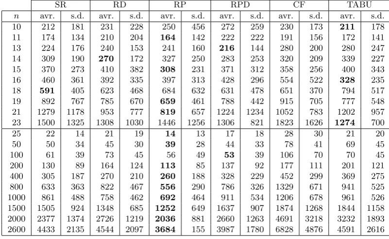
TABLE 1. The average execution time (avr.) and the standard deviation (s.d.) in millisecond of 50 trials to construct magic squares of different orders (n)

SR RD RP RPD CF TABU

n avr. s.d. avr. s.d. avr. s.d. avr. s.d. avr. s.d. avr. s.d.

10 212 181 231 228 250 456 272 259 230 173 211 178

11 174 134 210 204 164 142 222 222 191 156 172 141

13 224 176 240 153 241 160 216 144 280 200 280 247

14 309 190 270 172 327 250 283 253 320 209 339 227

15 370 273 410 382 308 231 371 312 358 256 400 343

16 460 361 392 335 397 313 428 296 554 522 328 235

18 591 405 623 468 684 632 631 478 651 370 794 517

19 892 767 785 670 659 461 788 442 915 705 777 548

21 1279 1178 953 777 819 657 1224 1234 1052 783 1202 957

23 1500 1325 1308 1030 1446 1256 1306 821 1823 1626 1274 700

25 22 14 21 19 14 13 17 18 28 30 21 20

50 50 34 45 30 39 28 44 33 78 41 69 45

100 61 39 73 45 56 49 53 39 106 70 70 45

200 130 89 164 124 113 85 137 92 177 111 201 121

400 305 187 270 210 260 188 328 229 452 299 369 275

800 633 363 822 467 556 290 786 326 1329 671 941 525

1000 861 488 758 462 692 464 911 534 1206 678 961 526

1500 1505 924 1348 685 1252 649 1637 907 1874 1268 1844 1158

2000 2377 1374 2726 1219 2036 881 2660 1263 4691 3218 3232 1893

2600 4433 2135 4544 2097 3684 155 3987 1780 6828 4876 4591 2616

4.3. Comparison of RP to the Best Known Heuristic Approach

Table 3 summarises the performance comparison of RP to the best previously proposed solution methodology (LAHC) which is the winner of the magic squares competition on some selected instances of order n. The RP based hyper-heuristic outperforms the LAHC approach in all the performance measures, including average execution time, maximum and minimum time in millisecond for all n. Moreover, the standard deviation associated with the average execution time of RP is lower than LAHC in all cases.

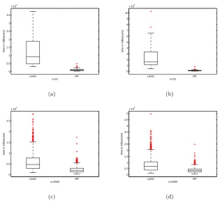
Figure 2 provides the sample box plots of run times obtained by LAHC and RP for the problem whenn=21, 23, 2000 and 2600. The Mann-Whitney-Wilcoxon test confirms that the RP based hyper-heuristic performs significantly better than the LAHC approach within a confidence interval of %95 for any givenn.

The inclusion of multiple low level heuristics and the stochastic nature of the hyper-heuristic makes it extremely difficult to compute the running time complexity of the overall algorithm. Hence, a regression model is formed based on largen. 50 trials to construct magic square of various orders form n=1000 to 2900 with increments of 100 have been considered for the regression model. Table 4 provides the Root Mean Square Error (RMSE) to indicate the quality of the fit. The random permutation based hyper-heuristic and the LAHC runs in O(n) time. RP has a smaller constant multiplier and RMSE values when compared to LAHC, showing that RP runs predictably faster than LAHC.

A final set of experiments are performed to observe

TABLE 4. Regression models to predict the running time complexity of the random permutation hyper-heuristic and the RMSE.

Apprach General Model Coefficients RMSE

RP a·n a= 1.359 1523

LAHC a·n a= 3.311 4745

the behaviour of RP and LAHC approach for the instances of orders n=21, 23, 2000 and 2600 varying the placement of the upper left-hand corner of the sub-matrix S3×3 at (i, j). We generated 100 and 2000 random locations of (i, j) for smalln=21, 23 and large

n=2000, 2600, respectively. Figure 3 provides the box plots obtained from LAHC and RP for their running times showing that RP still performs significantly better than the LAHC approach for thosenvalues.

4.4. A Performance Analysis of Low Level Heuristics under RP

Different low level heuristics contribute to the improvement of a solution in hand at different levels.

0 0.5 1 1.5 2 2.5 3 3.5 4 4.5 5

x 104

n=21

time in millisecond

LAHC RP

(a)

0 2 4 6 8 10

x 104

n=23

time in millisecond

LAHC RP

(b)

0 2000 4000 6000 8000 10000 12000 14000 16000

n=2000

time in millisecond

LAHC RP

(c)

0 0.5 1 1.5 2 2.5

x 104

n=2600

time in millisecond

LAHC RP

(d)

FIGURE 2. Box plots of execution time (in millisecond) from 50 runs for each hyper-heuristic constructing a constrained magic square for (a)n=21, (b) 23, (c) 2000 and (d) 2600.

0 0.5 1 1.5 2 2.5 3 3.5

x 104

n=21

time in millisecond

LAHC RP

(a)

0 1 2 3 4 5 6 7 8 9 10

x 104

n=23

time in millisecond

LAHC RP

(b)

0 0.5 1 1.5 2 2.5

x 104

n=2000

time in millisecond

LAHC RP

(c)

0 0.5 1 1.5 2 2.5 3 3.5 4 4.5 5

x 104

n=2600

time in millisecond

LAHC RP

(d)

TABLE 3. The average execution time (avr.), the standard deviation (s.d.), the maximum (max.) and the minimum (min.) in millisecond over 50 trials to construct magic squares of different orders (n)

LAHC RP

n avr. s.d. max. min. avr. s.d. max. min.

10 3825 3221 13717 955 250 456 3204 41

11 3409 4070 21623 1104 164 142 649 23

13 4823 4595 26268 1282 241 160 842 41

14 7841 8284 45049 1823 327 250 1197 71

15 7026 5603 25355 2170 308 231 1029 87

16 8356 8106 39394 2162 397 313 1544 112

18 8268 5905 23708 2652 684 632 2950 154

19 11325 10572 57327 2966 659 461 2463 165

21 16061 12340 48495 3640 819 657 3140 279

23 27399 25735 111373 4434 1446 1256 7210 267

25 157 26 214 90 14 13 61 1

50 366 252 1595 229 39 28 122 6

100 415 351 1622 195 56 49 305 8

200 1249 1140 6377 364 113 85 395 13

400 1790 1498 6700 456 260 188 750 36

800 3960 2722 12628 533 556 290 1396 117

1000 4620 2775 11088 724 692 464 2265 141

1500 5676 3957 16717 889 1252 649 3304 316

2000 6161 3822 16570 1166 2036 881 4572 579

2600 8142 4971 25284 1628 3684 1559 7126 1099

be that useful at the first glance, but considering that a portion of the worsening moves are accepted after the application of this low level heuristic, it seems to serve as a ”good” diversification component possibly in combination with the other heuristics. Figure 4 provides the utilisation rate of each low level heuristic considering improving moves only using a sample run forn=21, 23, 2000 and 2600. Under RP, each low level heuristic is invoked 50% of the overall time for large

n, but LLH1 achieved more improvement than LLH2. Moreover, it has been observed in almost all cases that 60-65% and 35-40% of the moves are improving when LLH1 and LHH2 are used, respectively.

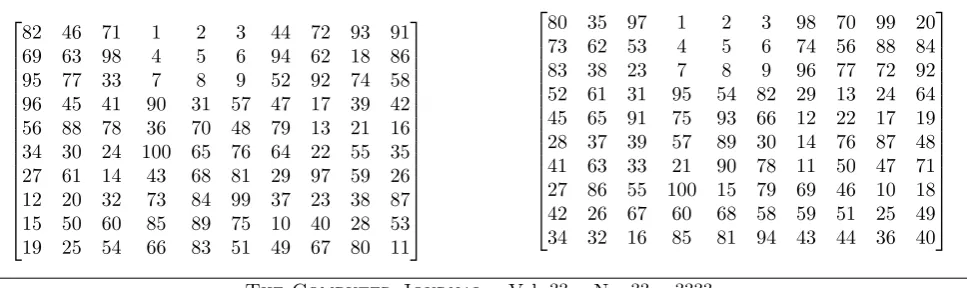
It is possible to obtain different magic squares of a given order. The following squares are the examples of two constrained version of magic square of order 10 generated by the described hyper-heuristic approach:

               

82 46 71 1 2 3 44 72 93 91 69 63 98 4 5 6 94 62 18 86 95 77 33 7 8 9 52 92 74 58 96 45 41 90 31 57 47 17 39 42 56 88 78 36 70 48 79 13 21 16 34 30 24 100 65 76 64 22 55 35 27 61 14 43 68 81 29 97 59 26 12 20 32 73 84 99 37 23 38 87 15 50 60 85 89 75 10 40 28 53 19 25 54 66 83 51 49 67 80 11

                LLH1 39% LLH2 4% LLH3 5% LLH4 34% LLH5 0% LLH6 3% LLH7 7% LLH8 0% LLH9 8% (a) LLH1 45% LLH2 3% LLH3 4% LLH4 35% LLH5 1% LLH6 3% LLH7 4% LLH8 0% LLH9 5% (b) LLH1 62% LLH2 38% (c) LLH1 62% LLH2 38% (d)

FIGURE 4. Utilisation rates of the low level heuristics based on improving moves only for (a) n=21, (b) 23, (c) 2000, and (d) 2600.

               

80 35 97 1 2 3 98 70 99 20 73 62 53 4 5 6 74 56 88 84 83 38 23 7 8 9 96 77 72 92 52 61 31 95 54 82 29 13 24 64 45 65 91 75 93 66 12 22 17 19 28 37 39 57 89 30 14 76 87 48 41 63 33 21 90 78 11 50 47 71 27 86 55 100 15 79 69 46 10 18 42 26 67 60 68 58 59 51 25 49 34 32 16 85 81 94 43 44 36 40

               

5. CONCLUSION

Hyper-heuristics have been shown to be effective solution methods across many problem domains. It has been observed that the performance selection hyper-heuristics may vary depending on the choice of heuristic selection and move acceptance components. [9] showed that the move acceptance is more influential on the performance of a selection hyper-heuristic if the number of low level heuristics is low and they are mutational. Then, the choice of move acceptance component becomes more crucial. In this study, different hyper-heuristics combining different selection and move acceptance methods are implemented as search methodologies to solve the constraint magic square problem. Unlike previous studies on hyper-heuristics, the performance of a hyper-heuristic is measured with its run-time rather than the quality of solutions obtained for the given problems. Still, the results confirm the previous observations. The random permutation based selection hyper-heuristic combined a na¨ıve acceptance method (RP−N AM) turns out to be an extremely effective and efficient approach which runs faster than all other hyper-heuristics using different move acceptance methods. Learning requires time slowing down a selection heuristic and so hyper-heuristics with no learning using the na¨ıve acceptance method are more successful than the learning hyper-heuristics regardless of whether the learning occurs within the heuristics selection or move acceptance component. RP −N AM outperforms the best known heuristic approach based on Late Acceptance for constructing a constrained magic squares.

REFERENCES

[1] Burke, E. K., Hart, E., Kendall, G., Newall, J., Ross, P., and Schulenburg, S. (2003) Hyper-heuristics: An emerging direction in modern search technology. In Glover, F. and Kochenberger, G. (eds.), Handbook of Metaheuristics, pp. 457–474. Kluwer.

[2] Burke, E., Hyde, M., Kendall, G., Ochoa, G., ¨Ozcan, E., and Woodward, J. (2009) A classification of hyper-heuristics approaches. Handbook of Metaheuristics. Springer - in press.

[3] Burke, E. K., Hyde, M. R., Kendall, G., Ochoa,

G., Ozcan,¨ E., and Woodward, J. R. (2009)

Exploring hyper-heuristic methodologies with genetic

programming. In Kacprzyk, J., Jain, L. C.,

Mumford, C. L., and Jain, L. C. (eds.),Computational Intelligence, Intelligent Systems Reference Library, 1, pp. 177–201. Springer Berlin Heidelberg.

[4] Ross, P. (2005) Hyper-heuristics. In Burke,

E. K. and Kendall, G. (eds.), Search Methodologies: Introductory Tutorials in Optimization and Decision Support Techniques, chapter 17, pp. 529–556. Springer. [5] Cowling, P., Kendall, G., and Soubeiga, E. (2001) A hyperheuristic approach to scheduling a sales summit. Selected papers from the Third International Conference on Practice and Theory of Automated Timetabling, London, UK, pp. 176–190. Springer-Verlag.

[6] Fisher, H. and Thompson, G. L. (1963) Probabilistic learning combinations of local job-shop scheduling

rules. In Muth, J. F. and Thompson, G. L.

(eds.),Industrial Scheduling, New Jersey, pp. 225–251. Prentice-Hall, Inc.

[7] ¨Ozcan, E., Bykov, Y., Birben, M., and Burke, E. (2009) Examination timetabling using late acceptance hyper-heuristics. Evolutionary Computation, 2009. CEC ’09. IEEE Congress on, may, pp. 997 –1004.

[8] Pisinger, D. and Ropke, S. (2007) A general heuristic

for vehicle routing problems. Computers and

Operations Research,34, 2403– 2435.

[9] ¨Ozcan, E., Bilgin, B., and Korkmaz, E. E. (2008) A comprehensive analysis of hyper-heuristics. Intelligent Data Analysis,12, 3–23.

[10] Bilgin, B., Ozcan,¨ E., and Korkmaz, E. (2007) An experimental study on hyper-heuristics and final exam scheduling. Practice and Theory of Automated Timetabling VI, pp. 394–412. Springer.

[11] Xie, T. and Kang, L. (2003) An evolutionary algorithm for magic squares. Evolutionary Computation, 2003. CEC ’03. The 2003 Congress on, dec., pp. 906 – 913.

[12] Burke, E. K. and Bykov, Y. (2012) The late

acceptance hill-climbing heuristic. Technical Report Technical Report No. CSM-192. Computing Science and Mathematics, University of Stirling.

[13] Burke, E. K. and Bykov, Y. (2008) A Late Acceptance

Strategy in Hill-Climbing for Exam Timetabling

Problems. PATAT ’08 Proceedings of the 7th

International Conference on the Practice and Theory of Automated Timetabling.

[14] Abuhamdah, A. (2010) Experimental result of late acceptance randomized descent algorithm for solving course timetabling problems. IJCSNS-International Journal of Computer Science and Network Security,10, 192–200.

[15] Verstichel, J. and Vanden Berghe, G. (2009) A late acceptance algorithm for the lock scheduling problem. In Voss, S., Pahl, J., and Schwarze, S. (eds.),Logistik Management, pp. 457–478. Physica-Verlag HD. [16] Nareyek, A. (2003) Choosing search heuristics by

non-stationary reinforcement learning. In Resende, M. G. C. and de Sousa, J. P. (eds.), Metaheuristics: Computer Decision-Making, chapter 9, pp. 523–544. Kluwer.

[17] ¨Ozcan, E. and Kheiri, A. (2012) A hyper-heuristic based on random gradient, greedy and dominance. In Gelenbe, E., Lent, R., and Sakellari, G. (eds.), Computer and Information Sciences II, pp. 557–563. Springer London.

[18] Burke, E. K., Kendall, G., and Soubeiga, E. (2003) A tabu-search hyperheuristic for timetabling and rostering. Journal of Heuristics,9, 451–470.

[21] Burke, E. K., Gendreau, M., Hyde, M., Kendall, G., Ochoa, G., ¨Ozcan, E., and Qu, R. (2013) Hyper-heuristics: A survey of the state of the art. Journal of the Operational Research Society, to appear,?

[22] Fagerland, M. W. and Sandvik, L. (2009) The

wilcoxon–mann–whitney test under scrutiny. Statistics in Medicine,28, 1487–1497.

[23] Kruskal, W. H. (1957) Historical notes on the wilcoxon unpaired two-sample test. Journal of the American Statistical Association,52, pp. 356–360.