Inferential framework for two-fluid model of cryogenic chilldown
DG Luchinsky∗, M Khasin
SGT, Inc., Greenbelt, MD, 20770, USA
D Timucin
Ames Research Center, Moffett Field, CA, 94035, USA J. Sass, B Brown
Kennedy Space Center, Kennedy Space Center, FL, 32899, USA
Abstract
We report a development of probabilistic framework for parameter inference of cryogenic two-phase flow based on fast two-fluid solver. We introduce a concise set of cryogenic correlations and discuss its parameterization. We present results of application of proposed approach to the analysis of cryogenic chilldown in horizontal transfer line. We demonstrate simultaneous optimization of large number of model parameters obtained using global optimization algorithms. It is shown that the proposed approach allows accurate predictions of experimental data obtained both with saturated and sub-cooled liquid nitrogen flow. We discuss extension of predictive capabilities of the model to practical full scale systems.
Keywords: Cryogenic flow, chilldown, two-phase flow, optimization, flow boiling, heat transfer.
1. Introduction
Autonomous management of two-phase cryogenic flows is a subject of great interest to many spacefarers including effective human exploration of the Solar Sys-tem [1, 2, 3]. It requires development of models that can recognize and predict cryogenic fluid dynamics on-line in nominal and off-nominal (i.e. in the presence of mass/heat leaks in the pipe etc.) flow regimes without human interaction.
However, predicting the behavior of two-phase flows is a long standing problem of great complexity [4, 5]. It becomes especially challenging when flowing fluids are far away from thermal equilibrium (e.g. during chill-down) and the analysis has to include heat and mass transfer correlations [6, 7, 8, 9].
During past decades a number of efficient algo-rithms [6, 10, 11, 12] and advanced correlation relations for heat and mass transfer [6, 13, 14] have been devel-oped for analysis of multi-phase flows [5, 9, 15, 16, 17]. Despite this progress the state of the art in two-phase
modeling lacks a general agreement regarding the fun-damental physical models that describe the complex phenomena [12]. As a consequence, uncertainties in modeling source terms may ultimately have a bigger im-pact on the results than the particular numerical method adopted [4].
Analysis of cryogenic fluids introduces further com-plications due to relatively poor knowledge of heat and mass transfer correlations in boiling cryogenic flows [18, 19, 20, 21, 22, 23]. Even less is known about flow boiling correlations of cryogenic fluids in micro-gravity [3, 24]. To address these and other mission crit-ical issues NASA has developed and implemented an impressive program of research, see e.g. [1, 2, 25, 26], that resulted in emergence of space based fluid manage-ment technologies.
commer-cially available for analysis of the model parameters and data correlations [38].
However, small time steps and instabilities [27, 37] or implicitness of numerical scheme [39, 40] impose substantial limitations on the speed of the solution, effi -ciency of multi-parametric optimization, and possibility of on-line application. As a result accurate predictions of transient cryogenic flows remain a challenge [23, 38] and extensive research is currently under way [3, 22].
Some of the grand challenges of this analysis include inference of parameters of cryogenic correlations from experimental time-series data and extension of the re-sults obtained from small experimental subsystems to full scale practical systems.
In this paper we report on the development of sepa-rated two-fluid model suitable for fast on-line analysis of cryogenic flows and introduce model-based inferen-tial framework capable of efficient multi-parametric op-timization of the model parameters.
We demonstrate an application of this inferential framework to the problem of modeling chilldown in horizontal cryogenic line. This problem has been shown to be a difficult one to solve in the earlier research [38]. Using proposed approach we obtain accurate predic-tions for transient liquid nitrogen flow both under sub-cooled and saturated conditions.
The paper is organized as follows. In the next Sec-tion we briefly describe the model and algorithm of its integration. In the Section 3 we introduce probabilis-tic framework for inference of the model parameters, discuss the uncertainties in the source terms and their parameterization. In the Section 4 we introduced con-stitutive relations used to model source teams. The ap-proach to the inference of model parameters is discussed in Section 5. In the Section 6 we describe an applica-tion of the proposed technique to an analysis of cryo-genic chilldown in horizontal pipe. Finally, in the Con-clusions we summarize the obtained results and discuss directions of future work.
2. Model
We limit our analysis to one-dimensional flow net-works having in mind fast on-line applications of the solver. To this end we have developed and tested a num-ber of algorithms [41, 42, 43, 44, 45, 46, 47, 48]) to see if their speed and accuracy can satisfy requirements of real-time application. It was shown that the nearly-implicit algorithm, similar to one developed in [10], can be applied successfully for on-line predictions of non-homogeneous (ug ,ul) and non-equilibrium (Tg ,Tl) flows.
In this section we will describe briefly the corre-sponding model equations and the algorithm of their in-tegration. Extensive details can be found in [41, 42, 49, 43], see also [47, 48].
2.1. Model Equations
In nearly implicit algorithm a closed system of equa-tions is obtained assuming equal local pressure values for the both phases [11, 50, 15]. The corresponding six-equation model consists of a set of conservation laws for the mass, momentum, and energy of the gas (see e.g. [10, 51, 6, 41, 42] )
(
Aαρg
) ,t+
(
Aαρgug
) ,x=AΓg
(
Aαρgug
) ,t+
(
Aαρgu2g
)
,x+Aαp,x=−Aαgρgz,x
−τgwlwg−τgili+AΓguig
(
AαρgEg
) ,t+
(
AαρgEgug
)
,x=−Apα,t−
(
pAαug
) ,x +q˙gwlwg+q˙gili+AΓgHg
(1)
and liquid phases
(Aβρl),t+(Aβρlul),x=−AΓg (Aβρlul),t+
(
Aβρlu2l
)
,x+Aβp,x=−Aβgρlz,x−
τlwlwl−τlili−AΓguil
(AβElρl),t+(AβElρlul),x=−Apβ,t−(pAβul),x+ ˙
qlwlwl+q˙lili−AΓgHl.
(2)
Herep,α,T, andρare pressure, temperature, and den-sity of the fluid. E is the total specific energy, Hg(l) is
the specific enthalpy of the gas generated (liquid evap-orated) at the interface and near the wall,gis the gravi-tational acceleration,uis the fluid velocity,τis the wall shear stress, and ˙q is the heat flux per unit area at the wall and at the interface. The total mass flux per unit volumeΓg= Γwg+ Γighas two components correspond-ing to the mass transfer at the wallΓwgand at the inter-faceΓig.
The fluid dynamics equations are coupled to the equa-tion for the wall temperatureTw
ρwcwdw∂∂Ttw =hwg
(
Tg−Tw
)
+hwl(Tl−Tw)+hamb(Tamb−Tw).
(3)
Hereρ,c, anddare density, specific heat, and thickness of the pipe wall,his the heat transfer coefficient corre-sponding to the ambient (hamb) and internal heat flowing to the wall from the gas (hwg) and liquid (hwl) phases.
The characteristic feature of the model (1), (2) is its non-hyperbolicity [15, 52] related to the assumption of exclusively algebraic terms describing the interfacial drag and incomplete formulation for the interfacial mo-mentum coupling. It can be shown that this system does
not have a complete set of real eigenvalues and does not represent a well-posed system of equations [41, 51, 53]. It is also known that this system displays lack of positivity and instabilities due to phase appear-ance/disappearance process [11, 54]. In addition, the effect of algebraic source terms represents a system of “stiff” differential equations [15] and roundoff errors may significantly contribute to numerical instabilities.
Despite these difficulties a number of algorithms were developed [6, 10, 11] and successfully employed to predict two-phase flows of boiling water in large scale system. In our development of the algorithm we were following the guidelines of earlier research.
2.2. Algorithm
The choice of the algorithm was guided by the fact [11] that all current reactor thermal-hydraulics codes [6, 10, 55] originate from Liles and Reed [56] ex-tension of Harlow and Asden [57, 58] all-speed implicit continuous-fluid Eulerian algorithm. These codes en-hance the stability of the method and eliminate material CFL restrictions using a couple of extensions: stability-enhancing two-step [6] and nearly implicit [10] algo-rithms.
In this work the discretization and integration of the model equations (1) - (3) follow closely the nearly-implicit method described in RELAP5-3D [10] (see [42, 47] for the details). The integration was performed in two steps. The first step of the algorithm can be briefly summarized as follows: (i) Solve expanded equation with respect to pressure expressed in terms of new ve-locities; (ii) Solve momenta equations written in the form of block tri-diagonal matrix for the new velocities; (iii) Find new pressure; (iv) Find provisional values for energies and void fractions using expanded equations of states; (v) Find provisional values of mass fluxes and heat transfer coefficients using provisional values of temperatures obtained.
At the second step new values of the densities, void fractions, and energies are found by solving the unex-panded conservation equations for the phasic masses and energies using provisional values for the heat and mass fluxes in source terms. The solution is reduced to independent solution of four tri-diagonal matrices. The values of pressure and velocities in these matrices are taken at the new time step.
The resulting scheme is efficient and fast and can in-tegrate 1000 sec of real time chilldown in a few seconds of computational time. For a model consisting ofN con-trol volumes it involves inversion of N 4×4 matrices, solution of 2×(N−1) tree-block-diagonal matrix
equa-tion, solution of fourN×Ntridiagonal matrix equations, andN×mexplicit computations.
A special attention was paid to the stability of the code. Various methods are available for regularization of the solution including standard upwinding and stag-gered grid methods as well as ad hoc smoothing and multiple time step controls techniques, see [42] for the details. Specifically, multiple techniques can be used to suppress [10, 52] the non-hyperbolicity.
In this work to suppress the non-hyperbolicty we are using so-called virtual mass term [10]
MV =Cαβρm
∂
(
ug−ul
)
∂t +ul
∂ug
∂x −ug
∂ul
∂x
in the right hand sides of the momentum equations. In practical computations the terms corresponding to spa-tial derivatives were neglected.
The stability of the algorithm was further enhanced by using the time step control to insure that all the ther-modynamic variables remain within the predetermined limits and that the change of these variables at any given time step does not exceed 25% of their values obtained at the previous time step. If these conditions are not sat-isfied the time step is halved and integration is repeated. If time step goes beyond limiting value the integration is terminated.
Similar control is applied to enforce mass conser-vation in each control volume and in the system as whole. In addition, smoothing mentioned above was found to be a very important tool to ensure stability of the scheme. In this work we followed recommendations provided by Liou [59] and adjust temperature, velocity, and density according to the following expression
ϕad j =g(x)ϕd+(1−g(x))ϕc, (4)
where
g(x)=x2(2x−3) ; and x= αd−xmin xmax−xmin.
Here “d” stands for disappearing phase and “c” for con-ducting phase. The exact values of the minimum and maximum void fraction xmin andxmaxwere established
using extensive numerical experimentation as∼ 10−7 and∼10−2respectively.
It is, therefore, important that the cryogenic modeling is embedded within optimization framework that allows efficient inference of the correlation parameters and sys-tematic comparison between various functional forms of the constitutive relations.
We note that corresponding optimization framework is also one of the key tools required for autonomous control of cryogenic flows. Accordingly in the current work we were focused on development of an efficient optimization framework. Below we briefly outline this approach.
3. Probabilistic framework
The most time consuming step in development of the cryogenic flow models is accurate correlation of the model predictions against experimental data (see e.g. [9] and references therein). This step is crucial for prac-tical applications of the model including e.g. reliable design of cryogenic hardware [38], analysis of nomi-nal regimes of operation, fault detection and isolation, and efficient recovery from off-nominal regimes. It be-comes even more important when one attempts to ex-tend model predictions to untestable conditions [38, 60] or to practical full-scale systems [61].
At present the main approach to correlation of exper-imental data is based on fitting (mainly by hand) exten-sive databases obtained in various flow regimes under carefully controlled experimental conditions [6, 62, 23]. The rationale behind this approach is an attempt to re-duced a very large number of uncertainties inherent to the model and to obtain solution of the fitting problem using traditional techniques.
However, such an approach becomes prohibitively expensive in development two-phase flow correlations and autonomous fluid management in microgravity. An efficient solution of the problem in this case has to rely on more intelligent and less expensive methods of infer-ring correlation parameters. This work is an attempt to establish feasibility of such methods. Below we briefly review the uncertainties of the model and outline prob-abilistic approach that can be applied to their analysis.
3.1. Uncertainties
Fundamentally, the probabilistic nature of the model predictions is related to the fact that the interface be-tween two phases is continuously fluctuating and nei-ther location nor the shape of the interface can be re-solved by the model. The spatial and time scales of these fluctuations are continuously changing depending on the flow regime. The intensity of these fluctuations is
especially significant during chilldown, when liquid and vapor phases coexist under strongly non-equilibrium conditions, see e.g. [31].
Another major source of uncertainty is related to the choice of the functional form of the correlations. There have been literally hundreds of various modifications proposed for the flow boiling correlations [63, 64] and the corresponding functional space is continuously ex-panding [22, 65]. In addition, the diversity of the cor-relations stems from the fact that there are several dif-ferent proposed physical flow and heat transfer mecha-nisms for each of the boiling regimes, see e.g. [3] for a review.
To illustrate this point let us consider as an example one of the key correlation parameters so-called critical heat flux, ˙qch f,0, corresponding to the maximum heat
transfer from boiling fluid to the wall.
One of the best known correlations for the pool boil-ing value of ˙qch f,0 was proposed by Zuber [66] in the
form
˙
qch f,0= π
24hlgρg
σg(ρl−ρg)
ρ2
g
1/4(
ρl
ρl+ρg
)1/2
.(5)
Zuber’s model assumes several approximations, includ-ing e.g. the followinclud-ing: (i) risinclud-ing jets with radiusRjform a square grid with a pitch equal to the fastest grow-ing wavelength due to Taylor instability, (ii) the risgrow-ing jets are assumed to have critical velocity dictated by Helmholtz instability, (iii) the neutral wavelength of the rising jet is assumed to be 2πRj.
It is clear from the list of assumptions that numerical constants in Zuber’s correlation have to be viewed only as an approximation. Furthermore, this approximation does not take into account surface wettability, pipe cur-vature, sub-cooling, and surface orientation. Accord-ingly, several corrections are known [9] that modify functional form of this correlation.
In boiling flows further corrections have to be intro-duced to take into account the dependence of the heat flux on the void fraction, velocity, and sub-cooling of the flow. For example, Griffith et all use the follow-ing functional form of the correspondfollow-ing corrections for cryogenic flows [67, 68]
˙
qch f = q˙ch f,0(αcr−α)
(
1+a1 (
ρlcl∆Tsub
ρghlg
)
(6)
+a2Rel+a3 (
Relρlcl∆Tsub
ρghlg
)1/2 ,
whereαcris the critical value of the void fraction and
ai are constants, e.g. a1 = 0.0144, a2 = 10−6, a3 =
0.5×10⁻³[69], andα
functional forms of similar corrections are also known and will be considered below.
In practice, we often used a simpler expression, cf [67, 70]
˙
qch f =q˙ch f,0·a1·(αcr−α)a2(1+a3Ga5), (7)
where typical values of parameters used in simulations area1=1.0,αcr=0.96,a2=2.0,a3=0.16, anda4=0.2.
Another source of uncertainty is added to the prob-lem by the fact that models are often correlated against multiple datasets obtained for different flow conditions. Some of these conditions (e.g. wettability) are not well known.
As a result of multiple approximations the number of parameters that have to be established in different flow regimes for practical full-scale systems is of the order of thousand. It becomes clear that computer base intel-ligent methods are required to handle complexity of this scale in realistic time frame.
3.2. Probabilistic approach
Here we consider briefly one of the approaches to the solution of this problem based on probabilistic Bayesian method [71]. Using this technique one can [71] estimate the probability of unknown model parameters
P(θ|d,m)= P(d|θ,m)P(θ|m)
P(d|m) , (8)
compare different models
P(d|m)= P(m|d)P(m)
P(d) (9)
and forecast system responsednto untested experimen-tal conditions
P(dn|d,m)=
∫
P(dn|θ,d,m)P(θ|d,m)dθ. (10)
Here,dis the experimental time-series data,mis the model, andθis the set of model parameters.
There are two important advantages of this approach to bear in mind. The first one is its ability to select sim-pler models over more complex models, thus resolv-ing so-called “Ockham’s razor problem” of optimiza-tion. The second advantage is its flexibility in the choice model parameters. It is known that the best predictive performance is often obtained [71] using the most flexi-ble system that can better adapt to the complexity of the data.
Accordingly, this approach allows for development of a flexible model with a set of parameters large enough to capture all the required properties of the data.
The main outcome of the method is distribution of the model parameters that contains maximum statistical information available in a given experimental data set. Importantly, this information can be updated when new time-series data or new database become available. As a result, the approach tends to provide the best fit to all available data.
3.3. Equivalent State Space Model
One of the key steps in developing probabilistic in-ferential framework is the solution of the optimization problem. In general terms this problem is formulated by presenting results of integration of equations (1) - (3) on one time steptin the form of discrete-time state-space model (SSM)
xt+1= f(xt,c)+εt,
yt=g(xt,b)+χt.
(11)
Here cis the set of the model parameters and xt is a
set of dynamical variables{ρg, ρl,Tg,Tl,ug,ul,p, α
}L t at timetdiscretized in space on a set of control volumes
VL.
The observationsytin the SSM are related to the un-observed states xt via nonlinear function g(xt,b). εt andχtin equations (11) are independent identically dis-tributed sources of Gaussian noise. The latter assump-tion is standard within this approach when sources of noise have multiple origin and are not well established (cf [71, 72, 73]).
Although it is possible to determine simultaneously parameter and state of a systems within proposed frame-work (see e.g. [71, 74, 73]), here for simplicity we ne-glect measurement noise and assume that the key dy-namical variables such as pressure ˆp, wall temperature
ˆ
Tw, and fluid temperature ˆTf can be measured directly in the experiment. This is indeed the case for the time-series data obtained during chilldown experiment at Na-tional Bureau of Standards [75] that will be considered below, see Sec. 6.
In the simplest case of general importance the prob-lem can be reduced to the curve fitting probprob-lem (cf [38]). The modelmin this case is the set of equations (1) - (3) completed with constitutive relations and equa-tions of state for the liquid and gas [10, 42]. Datad cor-respond to the time-series data{pˆ,Tˆf,Tˆw}of pressure, fluid and wall temperature obtained in the experiment.
θcorrespond to the model parameters that will be dis-cussed in more details in the following section.
of development and application of this approach to the analysis of chilldown in cryogenic horizontal line.
4. Constitutive relations
As was discussed above, the model (1) - (3) has to be completed with the equations of state and the constitu-tive relations. The equations of state can be included into the model in the form of NIST tables [42, 76]. Functional and parametric form of constitutive rela-tions, on the other hand, represent one of the main source of uncertainties in the model. The corresponding constitutive relations [49] define boundaries between flow and boiling regimes, interphase friction, the coef-ficient of virtual mass, wall friction, wall heat transfer, interphase heat and mass transfer.
In practical calculations the boundaries between flow and boiling regimes have to be determined first. Fric-tional losses and coefficients for the heat and mass trans-fer are defined at the next step for each flow regime.
In this work the boundaries between flow regimes are estimated using simplified Wojtan et al [77] map. The map was simplified in two ways. First we used only a few transition boundaries as shown below. Next, we estimated the location of these boundaries in the coordi-nates of mass flow rate ( ˙m) and vapor quality (χ) using original expressions. Finally, we approximated the lo-cation of these boundaries using low-dimensional poly-nomials and used polynomial coefficients as fitting pa-rameters.
The rationale behind approximate description of the boundaries of flow regimes is twofold. It is known [78] that Wojtan maps can only be considered as an approx-imation to the flow regimes for cryogenic fluids. In the experiments performed at NBS [75] the flow regimes were not established experimentally and therefore can-not be validated.
Stratified-Wavy-to-stratified transition.For the strati-fied to wavy stratistrati-fied transition flow on the plain ( ˙m, χ) we have
˙
mstrat=
(226.3)
2A
ldA2gdρg
(
ρl−ρg
)
µlg
χ2(1−χ)π3
1/3
+20χ,
where Agd and Ald are dimensionless cross-sectional area of the gas and liquid fractions.
Stratified-Wavy-to-annular-intermittent transition.
The transition boundary from wavy-stratified to annular or intermittent flow is given by the following relation
˙
mwavy=
{16A3
gdgDρlρg χ2π2
[
1−(2hld−1)2
].5
×[ π2
25h2
ld
(1−χ)−F1(q)(We Fr
)−F2(q)
l +1
]}.5
+50.
Here Wel and Frl are Weber and Froude numbers
(Wel =
˙
m2
lD
ρlσ andFrl = ˙
m2
l ρ2
lgD
), whilehld is dimension-less height of the liquid level.
Dryout transition that takes into account heat flux
from the wall has the form
˙
mdry=
[
4.25(ln(0.58 χ
)
+0.52) (ρgσ D
).17
×(gDρg
(
ρl−ρg
)).37(ρ l ρg
).25( 1 ˜
q
).7].93
.
Here ˜qis the heat flux at the wall normalized by the characteristic heat flux corresponding to the departure from nucleate boiling in the form [79]
qDN B=K·ρ1g/2hlg
[
σg(ρl−ρg
)]1/4
.
The location of these boundaries determines transi-tions between various regimes of heat transfer and pres-sure losses as will be discussed briefly below.
4.1. Heat and mass transfer
The total mass transferΓgin equations (1), (2) is the sum of the mass transfer at the wall and at the interface
Γg= Γwg+ Γig,
where
Γwg= ˙
qwl
Hg∗−Hl∗; Γig=
˙
qli+q˙gi
H∗g−Hl∗;
and
Hg∗−Hl∗=
{
Hg,s−Hl, Γ>0
Hg−Hl,s, Γ<0 .
The heat transfer correlations are subject of extensive research [7, 8]. Here we briefly outline a subset of these correlations selected in the present work. The heat fluxes at the wall and at the interface are defined as fol-lows
˙
qwg=hwg
(
Tw−Tg
)
; q˙ig=hig
(
Tl,s−Tg
)
; ˙
qwl=hwl(Tw−Tl) ; q˙il=hil
(
Tl,s−Tl
).
In the current work we are interested in relatively low mass fluxes,G<600kg/m2/s. In this limit correlations
for the heat flux are often based on the multiplicative or additive corrections to the values obtained for pool boiling [67, 68, 69, 66, 80]. The following heat trans-fer mechanisms are included in the analysis: (i) con-vection, (ii) nucleate boiling, (iii) transition boiling, (iv) film boiling, and (v) transition to dryout regime.
4.1.1. Convective Heat Transfer
Convective heat transfer in horizontal pipes distin-guishes four flow regimes: (F-L) forced laminar, (F-T) forced turbulent, (N-L) natural laminar, and (N-T) nat-ural turbulent convection. The corresponding correla-tions for the convective heat transfer can be taken in the form e.g. [6, 14]
hcb=
κ
Dh
4.36, F-L [63];
0.023·Re0.8Pr0.4, F-T [63];
0.1·(Gr·Pr)1/3, N-L [81];
0.59·(Gr·Pr)1/4, N-T [81].
(12)
HerePr=µCp
κ andGr= ρ
2gβ
T(Tw−Tl(g))D3
µ2 are Prandtl and Grashof numbers respectively, βT is the coefficient of thermal expansion, andDhis the hydraulic diameter. To guarantee a smooth transition between various regimes the maximum value ofhcbis taken as the value for the convective heat transfer.
We note that convective heat transfer in the stratified flow does not significantly affect the chilldown process, because the fluid temperature in this regime is close to (or lower than) saturation temperatureTs. The first crit-ical temperature that defines the shape of the boiling curve and influences the chilldown corresponds to the onset of nucleation boilingTonb.
4.1.2. Onset of nucleate boiling
The correlations for onset of nucleate boiling are based on the analysis of the balance between mechan-ical and thermodynammechan-ical equilibrium [9]. Using this analysis theTonb and the corresponding heat flux ˙qonb can be written in the form [82, 83, 84]
Tonb = Ts+F
1+
√
1+2∆Tsub
F
, (13)
˙
qonb =
B Pr2 ∆T
2
sat =hcb(Tonb−Tl) (14)
whereB = ρghlgκl 8σTs ,F =
hcbPr2l
2B ,∆Tsat =Tonb−Ts is the wall superheat, and∆Tsub=Ts−Tlis liquid subcooling temperature. The convective heat transfer coefficient is given by (12).
When the wall superheat exceeds∆Tsat = Tonb−Ts the nucleation boiling begins and the heat flux to the wall may increase by more than an order of magnitude significantly affecting the chilldown process. This in-crease continues until the heat flux approaches its criti-cal value ˙qch f.
4.1.3. Critical heat flux
The values of critical heat flux ˙qch f and the corre-sponding critical wall superheat Tch f are crucial for predicting chilldown and dryout phenomena in non-equilibriums flows. In nuclear reactor codes (see e.g. [14, 6]) these values are determined using look-up tables based on extensive experimental measurements obtained under various flow conditions. For cryogenic fluids experimental data remain sparse and values of
˙
qch f and Tch f are often estimated using mechanistic models, see e.g. [7, 9, 68, 85], see also [60] for a recent review.
The correlations for the critical heat flux where intro-duced in Sec. 3.1. The temperatureTch f for the critical heat flux was estimated in this work using approach pro-posed by Theler [86]
Tch f =
Ts
1−TsRg
hlg log(2kg+1)
, (15)
where kg is the isoentropic expansion factor that for ideal diatomic gases is 7/2 and Rg is the specific gas constant.
When wall superheat exceeds∆Tch f =Tch f −Ts, the transition boiling begins and the heat flux to the wall decreases sharply as a function of the wall temperature until the latter reaches minimum film boiling tempera-tureTm f b.
4.1.4. Minimum film boiling
In the film foiling regime the fluid flow is completely separated from the wall by the vapor film. The mini-mum value of the wall superheat ∆Tm f b = Tm f b−Ts corresponding to this regime was estimated by Beren-son as [87, 88]
∆Tm f b,0=0.127ρg
hlg κg × [
g(ρl−ρg) ρl+ρg
]2/3[ σ
g(ρl−ρg) ]1/2[
µg
(ρl−ρg)
]1/3 (16)
Iloeje [67, 70] has corrected Berenson equation to take into account the dependence of the ∆Tm f b on the quality and mass flux of the boiling flows in the form
∆Tm f b=c1∆Tm f b,0(1−c2Xec3)(1+c4Gc5), (17)
where Xe is the equilibrium quality, G is liquid mass flux andaiare constants, e.g. a1 =0.0144,a2 =10−6,
the film boiling regime was taken in the form of Brom-ley correlations
hbr =C·
gρgκ
2
g
(
ρl−ρg
)
˜
hlgcpg
D(Tw−Tspt
)
Prg
0.25
, (18)
corrected using Iloeje-type correlations [67, 70]
hf b=c1hbr(1−c2Xec3)(1+c4Gc5) (19)
Typical values of the parameters used in simulations are the following: (i)c1 =2.0; (ii)c2=1.04; (iii)c3 =2.0;
(iv)c4=0.2; (v)c5 =0.1.
The minimum film boiling heat flux can now be de-fined as
˙
qm f b=hf b∆Tm f b. (20)
To complete the discussion of the boiling heat trans-fer we notice that in the region of single phase gas flow the heat transfer is given by equations (12) with appro-priately modified parameters. Transition to the single phase heat transfer is initiated when dryout transition is detected.
4.2. Parametrization
It follows from the discussion above that boundaries between various flow boiling regimes are characterized by a number of critical points including onset of nucle-ate boiling, critical heat flux, minimum film boiling, and onset of dry-out. The heat flux to the wall at these points may differ by an order of magnitude.
To simplify the analysis of correlations in two-phase flow-boiling regimes the corresponding values of the heat flux can be anchored to the values at critical points as follows.
In the regime of nucleate flow boiling when the wall superheat increases from∆Tonbto∆Tch f. the heat flux can be defined using simple interpolation
˙
qnb=ynq˙onb+(1−yn) ˙qch f, (21)
wherenis constant,yis defined as (Tw−Tonb)/(Tch f −
Tonb), while ˙qch f and ˙qonbare given by the equations (6) and (14) respectively.
Similar correlations were applied to interpolate tran-sition boiling in the form [6]
˙
qtb= ftb·q˙ch f +(1−ftb) ˙qm f b, (22)
whereftb=
(
Tw−Tm f b Tch f−Tm f b
)2
, whereTch f,Tm f b, and ˙qm f bare
given by equations (15), (17), and (20) respectively. We note that ˙qch f is the same as in eq. (21) andTch f was
corrected using Iloeje-type correlations [70] similar to the one applied in eq. (17).
Within this approach the flow boiling correlations are essentially controlled by parameterization of the set of characteristic points on the boiling curve ccr =
{(Tonb,q˙onb), (Tch f,q˙ch f), (Tm f b,q˙m f b), (Tdry,q˙dry)}. By introducing corrections to temperature and heat transfer coefficient for critical heat flux and minimum film boil-ing in the form (17) and (19) we were able to obtain smooth transformation of the boiling surface between the pool and flow boiling regimes.
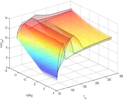
[image:8.595.324.530.327.493.2]An example of such transformation is shown in Fig. 1. In this figure the wall heat flux was calculated as a function of the wall temperature and Reynolds num-ber of the liquid nitrogen for three different values of pressure.
Figure 1: Heat flux from the liquid to the wetted wall as a function of the Reynolds number of the liquid flow and wall temperatureTw calculated for three different pressures: 1, 3, and 7 atm.
4.3. Pressure drop
To complete the discussion of the constitutive re-lations, we briefly consider pressure drop correlations used in this research.
For the single phase flow the wall drag was calculated using following relations
τwl= fwl
ρlu2l
2 , τwg= fwg
ρgu2g
2 , (23)
Here the friction factors for turbulent and laminar flow are given by Churchill approximation
fwg(l) =2 (
8
Re
)12
+ 1
(a+b)3/2
1/12
, (24)
with Reynolds numbers
Rem,L=
ρm,Lum,LDm,L
µg(l)
based on volume centered velocitiesum,Land hydraulic diameterDm = 4lAL
m,L for each control volume. Indexm
takes valuesm={g, l, i}for gas, liquid, and interface in a given control volume.
The coefficientsaandbhave the following form
a=2.475·log
1
(7
Re)
0.9
+0.27 (
ϵ Dh
)
16
,
b=(3.753Re×104)16.
The two-phase friction pressure drop (d pdz)
2ϕ is
de-fined using Lockhart-Martinelli correlations [90]. The pressure losses are partitioned between the phases as follows [10]
τwglwg=αg
(d p
dz
) 2ϕ
( 1 αg+αlZ2
)
, τwllwl=αl
(d p
dz
) 2ϕ
(
Z2
αg+αlZ2 )
.
HereZ2is given by
Z2=
(
fwlRelρlu2l
αwl
αl
)/ (
fwgRegρgu2g
αwg
αg
)
,
friction factor fwg(l)is in eq. (24), while coefficientsαwl andαwgdepend on the flow pattern [10].
The interface drag is given by
τig=−τil= 1
2CDρgug−ul(ug−ul
)
,
where interfacial drag coefficient CD depends on the flow pattern [6].
We note that the functional form of the correlations adopted in this work is not unique and a number of alter-native presentations can be used, see e.g. [14, 6, 91, 49] for further details. The main goal of the present analysis is to develop an efficient approach to the parameter in-ference and systematic comparison between alternative functional forms of these correlation.
5. Inference of the model parameters
The discussion in previous sections has emphasized the fact that modeling of cryogenic flows involves a large number of unknown parameters. We will now show that proposed probabilistic framework allows for their efficient simultaneous estimation.
The following steps are included into the process: (i) choice of the model parameters; (ii) definition of the ob-jective (cost) function; (iii) estimation of the initial dis-tribution of the model parameters via sensitivity study; (iv) simplified direct search for approximate globally optimized parameter values; (v) refined estimation of the optimal parameter values using global optimization; and (vi) estimation of the variance of the model param-eters.
5.1. Model parameters
Analysis of the correlations of the two-phase boiling flows in full scale industrial systems may involve hun-dreds of model parameters [14]. In the present simpli-fied model of the chilldown in horizontal straight line we limited studies to a set of 47 parameters divided into several groups, including e.g. parameters for: (i) on-set of nucleate boiling; (ii) critical heat flux; (iii) film boiling; (iii) convective heat transfer; (iv) flow regime boundaries; and (v) frictional losses.
For example, parameters related to the Iloeje’s cor-rections (19) to the minimum film boiling temperature
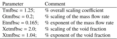
[image:9.595.311.536.444.519.2]Tm f bare combined in a group shown in Table 1. Simi-lar subsets of parameters were formed for other groups, see [49] for further details.
Table 1: Example of parameters for the temperatureTm f b.
Parameter Comment
Tmfbsc=1.25; % overall scaling coefficient Gtmfbsc=0.2; % scaling of the mass flow rate Etmfbsc=0.165; % exponent of the mass flow rate Xetmfbsc=2.0; % scaling of the void fraction Xtmfbsc=1.04; % exponent of the void fraction
Not all the parameters are equally important/sensitive for the system dynamics. Relative significance of the model parameters depends strongly on the objective of optimization, the stage of the chilldown process, and the location of the sensors in the system. Accordingly, the first step in the analysis of the sensitivity is an appropri-ate choice of the objective function.
5.2. Cost function
The primary goal of modeling large scale cryogenic systems is the ability to reproduce and predict sys-tem response in a variably of nominal and off-nominal regimes. The natural choice of the objective in this case is to minimize the sum of square difference between model predictions (xk
Typically, the fluid and wall temperatures and the fluid pressure are available for the measurements dur-ing chilldown. Takdur-ing into account time discretization of measured data, the cost function can be written in the form, cf. [38]
S(c)= N
∑
n=0
K
∑
k=1 [
ηTw (
Twk,n(c)−Tˆwk,n)2+ (25)
ηTf (
Tfk,n(c)−Tˆkf,n)2+ηp
(
pkn(c)−pˆkn)2
]
,
whereηiare weighting coefficients for different types of measurements, indexkruns through different locations of the sensors, and the indexncorresponds to discrete time instantst0, ...,tN.
5.3. Sensitivity analysis
[image:10.595.313.529.309.404.2]Once the objective function of optimization is chosen we proceed with the analysis of input-output relations for the model to determine the most sensitive model parameters. At this step we evaluate how much each model parameter is contributing into the model uncer-tainty.
Figure 2: Results of the sensitivity analysis forGwscexperimental time-series data obtained at NIST. Data recorded at different locations are shown by black solid lines for fluid temperature at three locations. Colored dashed lines show model predictions at: (red) 0.6m from the entrance; (blue) 24 m; (green) 43 m; (pink) 60 m
We perform this test for each motel parameter. An example of the test outcome for overall scaling coef-ficient for mass transfer at the wallGwsc is shown in Fig. 2. The sensitivity can be estimated as the relative change of the cost function normalized by the relative change of the parameter. In this particular example 12 % change in the parameter value results in 88 % change in the cost function, i.e. the sensitivity is considered to be very high, except for the data obtained at station 1.
The results of the sensitivity test were used primar-ily to simplify the model by fixing parameters that have no effect on the output and to rank the most sensitive parameters and to learn their effect on the output of the model at various sensor locations. Typically it was
found that only 20 parameters can be retained for sub-sequent model calibration.
5.4. Direct search
At the first step of the model calibration we used a simplified direct search to determine roughly the values of globally optimal model parameters.
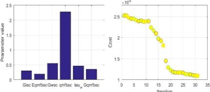
Simplified direct search algorithm developed in this work has proven to be highly efficient at this stage. The algorithm is searching for a minimum of the cost func-tion on a regular grid in multi-dimensional parameter space by scanning one parameter at a time. The search is repeated several times with randomly changing order of the scanning directions. The convergence of the al-gorithm is illustrated in the Fig. 3.
Figure 3: (a) Estimated values of the model parameters. (b) Con-vergence of the simplified direct search algorithm for simultaneous optimization of 6 model parameters.
In this example the following 6 parameters were ana-lyzed: scaling coefficients of the mass transfer at the in-terface (Gisc) and at the welted wall (Gwsc), character-istic time of the heat transfer to the wall (tauw), scaling coefficient for the film boiling heat transfer (qmfbsc), coefficientsc2(Gmfbsc) andc3(Emfbsc) in eq. (19) for
correction of the minimum heat flux.
The main advantage of this algorithm is that allows to determine quickly an approximate location of the global minimum in a given subspace of parameter space for poorly defined initial guess. tie: example, the algorithm can scan within one hour uo to 30 parameters of the NIST model using 10 different scanning orders.
An approximation to the values of the model param-eters found at this step can be further refined using one of the global optimization algorithms.
5.5. Global optimization
We note that casting the problem of fitting model predictions for two-phase flow in the standard form (11), (25) allows one to use any available standard li-brary for the solution of the optimization problem. In this work we performed global optimization using a
[image:10.595.65.285.402.498.2]set of optimization algorithms available in MATLAB. We have verified the convergence of the model pre-dictions towards experimental time series using pattern search, genetic algorithm, simulated annealing, and par-ticle swarm algorithms.
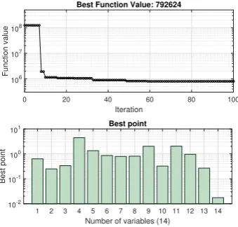
0 20 40 60 80 100
Iteration
106
107
108
Function value
Best Function Value: 792624
1 2 3 4 5 6 7 8 9 10 11 12 13 14
Number of variables (14)
10-2
10-1
100
101
Best point
Best point
Figure 4: (a) Convergence of the simulated annealing algorithm for simultaneous optimization of 14 model parameters. (b) Best values of the model parameters.
The convergence of the model predictions using sim-ulated annealing algorithm is illustrated in Fig. 4. We note that convergence is achieved for simultaneous op-timization of 14 parameters of the model. Besides 6 parameters listed above the following parameters were added to simultaneous optimization: scaling for the the Ditus-Boetler exponents in the heat transfer correlations on both sides of liquid vapor interface (hgi0esc and hli0esc) and at the dry wall (hg0esc), overall scaling for the heat transfer to the dry wall (hg0sc) and to the inter-face on the gas side (hgisc), scaling for the temperatures of the critical heat flux (Tchfsc) and minimum film boil-ing (Tmfbsc), and parameters of the transition boundary to the dispersed flow regime (xmin).
Once the estimation of the optimal values of the model parameters are refined we can formally complete inference procedure by estimating the variance of the model parameters.
5.6. Variance of the model parameters
To estimate variance we repeat optimization using lo-cal search with multiple restarts in the vicinity of the quasioptimal parameter value. Essentially, at this stage we enhance original sensitivity analysis using simplex algorithm.
[image:11.595.318.517.116.250.2]An example of estimation of the variance of param-eter value is shown in the Fig 5. In this example the distribution function for the parameter values obtained
Figure 5: Example of estimation of the variances of the parameter values obtained using local search with multiple restarts.
by direct calculations of the cost function for various values of the model parameter close to its optimal value are shown in figure by open symbols. The results of the direct numerical estimation of the distribution of the model parameters were fitted by Gaussian function
F=A(c0)·exp (
−1
2(c−c0)
∂2S(c 0)
∂c2 (c−c0) )
(26)
The results of the fitting are shown in the figure by thin solid lines. We note that the fit by Gaussian function is quite satisfactory close to the maximum of the dis-tribution. However, numerical simulations also reveal strong deviations from Gaussian fit for some values of the parameters. Specifically, analysis shows the range of parameter values were simulations diverge.
These results also provide enhanced sensitivity anal-ysis. For example, for parameter corresponding to the scale of the mass transfer coefficient at the wall (Gwsc) the dispersion σ2 ≈ 0.025 indicated the fact that the value of this parameter can be determined quite accu-rately using optimization procedure. On the other hand, the dispersion of the scaling coefficient of the heat trans-fer from the gas to the wall in the regime of forced con-vection (hg0sc) is very largeσ2 ≈ 12, indicating that
this parameter value can not be estimated accurately during optimization.
The described optimization procedure is robust and sufficiently fast. Simultaneous optimization of 14 model parameters for the NIST (see next section) model with 30 control volumes, including sensitivity analysis, di-rect search, and global optimization can be computed in several hours on the laptop.
[image:11.595.84.254.189.351.2]rough estimation of the distribution of the model pa-rameters and then we use available experimental time-series data to update these distributions by estimating globally optimal values of the model parameters and their variance. This procedure can be systematically continued as soon as new experimental data become available. Furthermore, various alternative functional forms of the two-phase flow correlations can be encom-passed and systematically compared with each other within proposed framework using data available in mul-tiple databases.
An important feature of the proposed approach is its flexibility and ability to impose sufficient number of constraints to guarantee physically valid solution of the optimization problem.
Firstly, we note that all the solutions satisfy (and therefore are consistent with) the fundamental con-servation laws of fluid dynamics given by equations (1). Secondly, all the correlations included into the model originate from the physics based analysis and corresponding bounds can be imposed on the value of each fitting parameter limiting its variation to physi-cally/experimentally relevant range. Thirdly, the values of the measured dynamical variables are anchored to the experimental time series by the choice of the cost func-tion (25).
In addition, the upper and lower bounds can be set for any hidden (not available for measurements) dynamical variable to keep its values within desired physical range. Also a penalty of arbitrary functional form can be added to the cost function (25) to ensure that values of specific parameter/variable are drawn form a given distribution. In the present research we adopted relaxed constraints that allow model parameters to deviate approximately 50% from the values reported in the literature. These constraints can be scrutinized in the future when more accurate time series data become available.
Using this approach we were able to demonstrate convergence of the model predictions towards experi-mental time-series obtained for chilldown of the cryo-genic transfer lines under various experimental condi-tions [48, 92, 93, 94, 95]. An example of such conver-gence is provided in the next section.
6. Application to cryogenic transfer line
To validate this approach we used a set of experimen-tal data obtained for chilldown in horizonexperimen-tal transfer line at National Bureau of Standards (currently NIST) [75] and chilldown large scale experimental transfer line at KSC [26]. Here we describe the result of the
appli-cation of our approach to the analysis of chilldown in NIST experiment.
In the chilldown experiment [75] the vacuum jack-eted line was 61 m long. The internal diameter of the copper pipe was 3/4 inches. Four measurement stations were located at the distance 6, 24, 42, and 60 m from the input valve. Three particular experimental data sets were considered in this work: (i) subcooled liquid ni-trogen and pressure in the storage tank was 4.2 atm; (ii) saturated liquid nitrogen flow driven by 3.4 atm pres-sure in the tank; and (iii) saturated liquid nitrogen flow driven by 2.5 atm pressure in the tank.
This set of experiments was selected for our analysis because it possesses a well-known difficulty for model-ing, see e.g. [38].
We note that there likely to be wall temperature dif-ference between the top and the bottom of horizontal tube for stratified flows. It is straightforward to include the corresponding phenomenon into the model since the fluid stratification is already embedded into two-phase flow dynamics ensuring that for stratified flow the bot-tom of the tube is filled with the liquid and the top with gas. However, adding wall tube stratification will re-sult in an over-fitting NIST data for the following rea-sons (to mention a few): (i) the accuracy of the supply pressure and the line temperature measurements is un-known; (ii) the exact initial temperature of the liquid is unknown; (iii) the material specification for the cop-per line is missing; (iv) the ID and roughness of the tube are uncertain; and (v) the temperature measurements are provided only at the bottom of the tube.
Due to these uncertainties, it is impossible to vali-date the model with the stratified wall temperature us-ing NIST data and a more complete data set will be re-quired to do it in the future. We note, however, that even very accurate measurements under well defined experi-mental conditions in a simple geometrical structure re-veal [34, 35] significant uncertainties in the system pa-rameters due to the nature of two-phase flow discussed above.
6.1. Sub-cooled flow
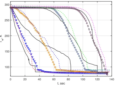
The results of modeling chilldown of cryogenic trans-fer line with sub-cooled liquid nitrogen flow under tank pressure 4.2 atm are shown in the next four figures. The corresponding time-series data include fluid and wall temperature, the heat flux coefficient, and fluid pressure. The results of comparison of the model predictions with the experimental data for the fluid temperature are shown in the Fig. 6. The corresponding comparison for the wall temperature is shown in the Fig. 7
0 20 40 60 80 100 120 140 t, sec
100 150 200 250 300
Tf
[image:13.595.78.260.119.263.2], K
Figure 6: Comparison of the model predictions (dashed colored lines) with the experimental time-series data (solid lines) for the fluid tem-perature measured at four locations along the pipe. Dashed colored lines and lines with colored open symbols correspond to the model predictions with two different sets of parameters.
Three different regions can be noticed in the figure. A fast cooling region in the beginning of the pipe. A region near the second station with long characteristic cooling time (order of 100 sec). And a region in the second half of the pipe that the remains hot for an ex-tended period of time.
0 20 40 60 80 100 120 140
t, sec 100
150 200 250 300
Tw
, K
Figure 7: Comparison of the model predictions (dashed lines) with the experimental time-series data (solid lines) for the wall temperature measured at four locations along the pipe. Color codding is the same as in previous figure.
It can be seen from the figure that all three regions are reproduced by the model quite accurately both for the fluid and wall temperature.
In general the solution of the optimization problem is not unique. Given different initial conditions the al-gorithm may converge to a slightly different values of
parameters. Example of such convergence to two diff er-ent sets of parameter values is illustrated in Figs. 6 to 9 by different color codding.
Both sets of parameters converged to the experimen-tal time-series data within accepted tolerance and corre-spond to sub-optimal values of the cost function (25).
0 20 40 60 80 100 120 140
t, sec 0
0.5 1 1.5 2 2.5
h, kW/m
[image:13.595.324.508.205.318.2]2/K
Figure 8: Comparison of the model predictions (dashed lines with open symbols) with the experimental time-series data (solid black lines) for the heat transfer coefficient measured at four locations along the pipe. Color codding is the same as in previous figures.
The non-uniqueness of the solution is a generic fea-ture of the two-phase flow models that stems from the complex landscape of the cost function with multiple local minima. Regularization of the solution can be achieved e.g. by measurements of the additional flow variables or by testing the flow under different flow con-ditions.
For example, the comparison of the model predic-tions with experimental time-series for the heat transfer coefficient and for the pressure are shown in Fig. 8 and Fig. 9 respectively.
0 50 100
t, sec
0 2 4 6 8
p1
, atm
0 50 100
t, sec
0 2 4 6 8
p2
, atm
0 50 100
t, sec
0 2 4 6 8
p4
, atm
[image:13.595.79.270.447.588.2] [image:13.595.317.525.545.663.2]It can be seen from the figures that experimentally estimated values of the total heat transfer coefficient to the wall are nearly constant at all locations and times ex-cept for a few narrow peaks. Therefore, the analysis of the heat transfer coefficient can provide in this case only semi-quantitative validation of the model predictions.
The comparison of the model predictions with ex-perimental time-series data for the pressure shown in Fig. 9 (note that the pressure time-series data are avail-able only at three locations) are more informative. The model can capture semi-quantitatively the frequency and the mean values of the pressure oscillations.
However, large amplitude oscillations of pressure sig-nal cannot be reproduce by the model. The most likely reason for this discrepancy is the dynamics of the in-put valve, which parameters are unknown. Therefore, during numerical experiments we usually limited con-tribution of the pressure signal to the cost function by setting values ofηpto∼0.1 in eq. (25).
6.2. Saturated flow
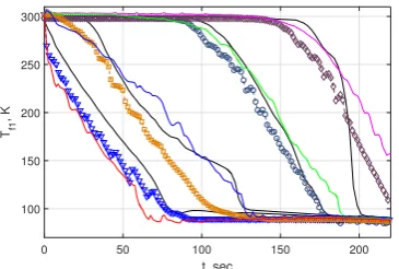
As was mentioned above the convergence of the may be further improved by extending analysis to encom-pass time-series data obtained under different flow con-ditions. Following this idea we have included into our analysis the time-series data obtained in NIST experi-ment [88] for saturated flows for two different driving pressures in the storage tank. Here we consider chill-down in the horizontal line observed for saturated nitro-gen flow driven by the tank pressure 3.4 atm, see Fig. 6.
0 50 100 150 200
t, sec 100
150 200 250 300
Tf1
[image:14.595.76.259.506.629.2], K
Figure 10: Comparison of the model predictions (dashed colored lines) with the experimental time-series data (solid lines) for the fluid temperature measured at four locations along the pipe. The nitrogen was under saturated conditions in the tank with pressure 3.4 atm.
It can be seen from the figure that the main effect of the reduced tank pressure (and corresponding reduction of nitrogen mass flow rate through the inlet valve) is an
increase of the chilldown time by approximately 70 sec. Note, that the shape of the temperature signals remains essentially the same, cf. Fig. 6.
A good agreement between model predictions and ex-perimental time-series data can be obtained using the same sets of the model parameters discussed above with small ( within 10% ) adjustment of parameter tauw. Similar results are obtained for saturated nitrogen flow under tank pressure 2.5 atm.
We note, however, that the uncertainty in the infer-ence of model parameters could not be resolved. We believe that the main reason for this is threefold: (i) the complexity of the temperature dynamics at the loca-tion of the 2-nd measurement staloca-tion; (ii) the limited set of correlations adopted in this work for modeling cryo-genic flow boiling during chilldown; and (iii) the limited information about system dynamics available in NIST time-series data. All these issues will be addressed in the future work in more details.
7. Conclusion
To summarize, we developed fast and reliable solver for separated two-fluid cryogenic flow based on nearly-implicit algorithm and proposed a concise set of cryo-genic two-phase flow boiling correlations capable of reproducing a wide range of experimental time-series data.
The main emphasis in this work were placed on de-velopment of an efficient algorithm for simultaneous learning of a large number of parameters of cryogenic correlations that could ensure convergence of the model predictions towards experimental time-series data.
Such an algorithm was proposed within inferential probabilistic framework. It involves the following steps: (i) sensitivity analysis of the model parameters, (ii) sim-plified direct search for approximate globally optimal values of these parameters, (iii) global stochastic op-timization that refines the estimate for parameter val-ues obtained at the previous step, and (iv) estimation of variance of the model parameters using local non-linear optimization.
The proposed approach was used to analyze chill-down in the horizontal transfer line with liquid nitro-gen flow. It was shown that the algorithm can reliably converge towards experimental time-series data in the space of∼20 model parameters both for sub-cooled and saturated flows.
At the same time the analysis revealed the non-uniqueness of inferred set of model parameters. The latter results indicates that to obtain more accurate and
reliable predictions the set of correlations will have to be extended and validated on a larger database of ex-perimental data. These issues will be addressed in the future work.
Another direction of future research will involve de-velopment an automation of the proposed approach us-ing machine learnus-ing framework.
It is important to note that the machine learning ap-proach will most likely underly autonomous control and fault management of two-phase flows in the future space missions. Therefore, its development may accelerate and improve both learning required correlation param-eters and reliable design of future exploration missions relying on two-phase flow management in space.
Acknowledgments
This work was supported by the Advanced Explo-ration Systems and Game Changing Development pro-grams at NASA HQ.
References
[1] D. J. Chato, Cryogenic fluid transfer for exploration, Cryogenics 48 (5-6) (2008) 206–209.
[2] W. Notardonato, Active control of cryogenic propellants in space, Cryogenics 52 (46) (2012) 236–242.
[3] C. Konishi, I. Mudawar, Review of flow boiling and critical heat flux in microgravity, International Journal of Heat and Mass Transfer 80 (2015) 469–493.
[4] A. Prosperetti, G. Tryggvason, Computational Methods for Multiphase Flow, Cambridge University Press, 2007.
[5] M. Ishii, T. Hibiki, Thermo-Fluid Dynamics of Two-Phase Flow, Springer, Bcher, 2010.
[6] United States Nuclear Regulatory Commission, TRACE V5.0 Theory Manual Field Equations, Solution Methods, and Physi-cal Models (2007).
[7] L. S. Tong, Y. S. Tang, Boiling Heat Transfer And Two-Phase Flow, Series in chemical and mechanical engineering, Taylor & Francis, 1997.
[8] A. Faghri, Y. Zhang, Transport Phenomena in Multiphase Sys-tems, Elsevier Science, 2006.
[9] S. Ghiaasiaan, Two-Phase Flow, Boiling, and Condensation: In Conventional and Miniature Systems, Cambridge University Press, 2007.
[10] Idaho National Laboratory, RELAP5-3D Code Manual Vol-ume I: Code Structure, System Models, and Solution Methods (2012).
[11] R. Nourgaliev, Solution Algorithms for Averaged Equations, Tech. Rep. INL/EXT-12-27187, Idaho National Laboratory (2012).
[12] R. A. Berry, J. W. Peterson, H. Zhang, R. C. Martineau, H. Zhao, L. Zou, D. Andrs, RELAP-7 Theory Manual, The Idaho Na-tional Laboratory, Idaho Falls, Idaho 83415 (2014).
[13] K. Y. Choi, B. J. Yun, H. S. Park, H. D. Kim, Y. S. Kim, K. Y. Lee, K. D. Kim, Development of a wall-to-fluid heat transfer package for the space code, Nuclear Engineering and Technol-ogy 41 (9) (2009) 1143–1156.
[14] Idaho National Laboratory, RELAP5-3D Code Manual Volume IV: Models and Correlations (2012).
[15] H. St¨adtke, Gasdynamic Aspects of Two-Phase Flow, WILEY-VCH Verlag, 2006.
[16] L. Wojtan, T. Ursenbacher, J. R. Thome, Investigation of flow boiling in horizontal tubes: Part ii - development of a new heat transfer model for stratified-wavy, dryout and mist flow regimes, International Journal of Heat and Mass Transfer 48 (14) (2005) 2970–2985.
[17] L. Cheng, G. Ribatski, L. Wojtan, J. R. Thome, New flow boil-ing heat transfer model and flow pattern map for carbon diox-ide evaporating insdiox-ide horizontal tubes, International Journal of Heat and Mass Transfer 49 (21-22) (2006) 4082–4094. [18] N. T. Van Dresar, J. D. Siegwarth, M. M. Hasan, Convective
heat transfer coefficients for near-horizontal two-phase flow of nitrogen and hydrogen at low mass and heat flux, Cryogenics 41 (11-12) (2001) 805–811.
[19] H. Umekawa, M. Ozawa, T. Yano, Boiling two-phase heat trans-fer of ln2 downward flow in pipe, Experimental Thermal and Fluid Science 26 (6-7) (2002) 627–633.
[20] J. Jackson, Cryogenic two-phase flow during chilldown: Flow transition and nucleate boiling heat transfer, Ph.D. thesis, Uni-versity of Florida (2006).
[21] S. Wang, J. Wen, Y. Li, H. Yang, Y. Li, J. Tu, Numerical predic-tion for subcooled boiling flow of liquid nitrogen in a vertical tube with musig model, Chinese Journal of Chemical Engineer-ing 21 (11) (2013) 1195–1205.
[22] S. R. Darr, H. Hu, R. Shaeffer, J. Chung, J. W. Hartwig, A. K. Majumdar, Numerical Simulation of the Liquid Nitrogen Chill-down of a Vertical Tube, AIAA SciTech, American Institute of Aeronautics and Astronautics, 2015.
[23] J. W. Hartwig, J. Vera, Numerical Modeling of the Transient Chilldown Process of a Cryogenic Propellant Transfer Line, in: 53rd AIAA Aerospace Sciences Meeting, AIAA SciTech, American Institute of Aeronautics and Astronautics, 2015. [24] K. Yuan, Cryogenic boiling and two-phase chilldown process
under terrestrial and microgravity conditions, Ph.D. thesis, Uni-versity of Florida (2006).
[25] J. Kim, Review of Reduced Gravity Boiling Heat Transfer: US Research, J. Jpn. Soc. Microgravity Appl. 20 (4) (2003) 264– 271.
[26] R. Johnson, W. Notardonato, K. Currin, E. Orozco-Smith, In-tegrated Ground Operations Demonstration Units Testing Plans and Status, in: AIAA SPACE 2012 Conference & Exposition, SPACE Conferences & Exposition, American Institute of Aero-nautics and AstroAero-nautics, 2012.
[27] A. Hedayatpour, B. Antar, M. Kawaji, Analytical and numerical investigation of cryogenic transfer line chilldown, in: 26th Joint Propulsion Conference, Joint Propulsion Conferences, Ameri-can Institute of Aeronautics and Astronautics, 1990.
[28] M. Kawaji, Boiling heat transfer during quenching under micro-gravity, in: Fluid Dynamics Conference, Fluid Dynamics and Co-located Conferences, American Institute of Aeronautics and Astronautics, 1996.
[29] A. Majumdar, T. Steadman, Numerical Modeling of Ther-mofluid Transients During Chilldown of Cryogenic Transfer Lines, in: 33rd International Conference on Environmental Sys-tems, Vol. 3, Society of Automotive Engineers, Vancouver, B.C., 2003.
[30] A. K. Majumdar, S. S. Ravindran, Fast, nonlinear network flow solvers for fluid and thermal transient analysis, International Journal of Numerical Methods for Heat & Fluid Flow 20 (6-7) (2010) 617–637.