On the parallelization of atmospheric inversions of CO2 surface ﬂuxes within a variational framework

(1)

Geosci. Model Dev., 6, 783–790, 2013 www.geosci-model-dev.net/6/783/2013/ doi:10.5194/gmd-6-783-2013

EGU Journal Logos (RGB)

Advances in

Geosciences

Open Access

Natural Hazards

and Earth System

Sciences

Open Access

Annales

Geophysicae

Open Access

Nonlinear Processes

in Geophysics

Open Access

Atmospheric

Chemistry

and Physics

Open Access

Atmospheric

Chemistry

and Physics

Open Access

Discussions

Atmospheric

Measurement

Techniques

Open Access

Atmospheric

Measurement

Techniques

Open Access

Discussions

Biogeosciences

Open Access Open Access

Biogeosciences

Discussions

Climate

of the Past

Climate

of the Past

Discussions

Earth System

Dynamics

Earth System

Dynamics

Discussions

Geoscientific

Instrumentation

Methods and

Data Systems

Open Access

_{Geoscientific}

Instrumentation

Methods and

Data Systems

Open Access

Discussions

Geoscientific

Model Development

Geoscientific

Model Development

Discussions

Hydrology and

Earth System

Sciences

Open Access

Hydrology and

Earth System

Sciences

Open Access

Discussions

Ocean Science

Discussions

Solid Earth

Discussions

The Cryosphere

Discussions

Natural Hazards

and Earth System

Sciences

Open Access

Discussions

On the parallelization of atmospheric inversions of CO

2

surface

fluxes within a variational framework

F. Chevallier

Laboratoire des Sciences du Climat et de l’Environnement, CEA-CNRS-UVSQ, L’Orme des Merisiers, UMR8212, Bat 701, 91191 Gif-sur-Yvette, France

Correspondence to: F. Chevallier ([email protected])

Received: 14 November 2012 – Published in Geosci. Model Dev. Discuss.: 8 January 2013 Revised: 18 April 2013 – Accepted: 7 May 2013 – Published: 7 June 2013

Abstract. The variational formulation of Bayes’ theorem

al-lows inferring CO2sources and sinks from atmospheric

con-centrations at much higher time–space resolution than the en-semble or analytical approaches. However, it usually exhibits limited scalable parallelism. This limitation hinders global atmospheric inversions operated on decadal time scales and regional ones with kilometric spatial scales because of the computational cost of the underlying transport model that has to be run at each iteration of the variational minimiza-tion. Here, we introduce a physical parallelization (PP) of variational atmospheric inversions. In the PP, the inversion still manages a single physically and statistically consistent window, but the transport model is run in parallel overlap-ping sub-segments in order to massively reduce the compu-tation wall-clock time of the inversion. For global inversions, a simplification of transport modelling is described to con-nect the output of all segments. We demonstrate the perfor-mance of the approach on a global inversion for CO2with a

32 yr inversion window (1979–2010) with atmospheric mea-surements from 81 sites of the NOAA global cooperative air sampling network. In this case, we show that the duration of the inversion is reduced by a seven-fold factor (from months to days), while still processing the three decades consistently and with improved numerical stability.

1 Introduction

CO2 mole fractions in the atmosphere are functions of the

CO2surface fluxes, of the atmospheric transport fluxes and,

to a smaller extent, of the photochemical CO2 production

in the atmosphere. Inferring (or inverting) the surface fluxes

from mole fraction measurements is made challenging by the combination of these three inputs, but it is rigorously guided by the Bayesian paradigm. An additional complication lies in the diversity of the time–space scales that are involved. At one end, the exceptionally long mean life time of CO2

links any mole fraction measurement to global CO2surface

(2)

numerical weather prediction (NWP), the variational formu-lation of Bayes’ theorem was introduced in the mid-2000s to lift this restriction (Chevallier et al., 2005; R¨odenbeck et al., 2005), but it requires tedious initial developments (i.e. coding the adjoint of the atmospheric transport) and usually exhibits limited scalable parallelism (Hamrud, 2010).

This paper focusses on the technical performance of the variational approach. Chevallier et al. (2010) performed a global 21 yr inversion at grid point (3.75◦ longitude and 2.5◦latitude) and weekly scale with this approach, but they needed 6 weeks of sustained parallel computing – the par-allelization being for the code of the transport model. The high cost of this 21 yr inversion implies prohibitive costs for extended inversion periods, higher resolution transport mod-elling or more sophisticated physical parameterization of the transport model. Given the parallel structure of current su-percomputers, finding high levels of parallelism has become critical for the developers of the variational approach (see, e.g. Fisher et al., 2011; Desroziers and Berre, 2012, in the field of NWP). At present, this approach is intrinsically se-quential because it consists in iteratively minimizing a cost function, each iteration step relying on the results of the previous one. Higher resolutions of the transport models al-low parallelizing on more processors, but the gain offered by the latter never fully compensates for the cost of the for-mer because of communication overheads. Moreover, trans-port models perform a lot of input operations (e.g. to read the transport mass fluxes) that are not well parallelizable. This problem is even bigger for their adjoint codes that read most of the information about the linearization point from the disk. In this paper, we introduce a parallel structure of the trans-port computations within variational atmospheric inversion systems in order to massively reduce the computation wall-clock time, while still running the inversion on a single physically and statistically consistent window. This struc-ture defines an ensemble of parallel computations that does not carry any statistical meaning, in contrast to the above-mentioned ensemble methods. We call it physical paralleliza-tion (PP) here to distinguish it from the statistical methods. We illustrate the efficiency of the PP for a 32 yr inversion window (1979–2010) for CO2 with atmospheric

measure-ments from 81 sites of the NOAA global cooperative air sampling network. Section 2 introduces the PP. The inver-sion system and the measurements used to illustrate it are described in Sects. 3 and 4, respectively. The results are pre-sented in Sect. 5. Section 6 concludes the paper.

2 Physical parallelization

An inversion system operates within a temporal window starting at a chosen time T (for instance, 1 January 1979 at 00:00 UTC in Sect. 4). Within this window, the transport modelHsimulates the mole fraction measurements made at any timet from the surface fluxes existing between times

T andt and from the 3-D field of mole fraction at the initial timeT. In the case of regional inversions,Halso uses the lat-eral boundary conditions of the mole fractions between times T andt.

Variational inversion systems minimize a Bayesian cost function and, to this end, exploit a linearized version ofH, under the form of a tangent-linear code and of an adjoint code.

In the tangent-linear code of H, a perturbation in mole fraction caused by perturbations in surface fluxes, by pertur-bations in the lateral boundary conditions and by perturba-tions in initial mole fracperturba-tions, is computed as

δc(t )=Xt t0_=TH

ϕ

t0_t·δϕ(t0)+Hc_t0_t·δc(T ), (1) withδc(t )the vector that contains the mole fraction incre-ments at timet,δϕ(t0₎_{the vector that contains the flux} incre-ments and the lateral boundary condition increincre-ments at time t0, Hϕ_t0_tthe linear operator (Jacobian matrix) that linksδϕ(t

0₎

andδc(t ), and Hc_t0_t the linear operator that linksδc(T )and δc(t ). Note that in variational systems, the two Jacobian ma-trices are not explicitly computed: the multiplication by the input increment vector is obtained from the chain rule ap-plied to the reference code, line by line.

The PP brings a small simplification to Eq. (1) by reduc-ing the backward influence to a timeτ which is later thanT following

δc(t )=Xt t0_=τH

ϕ

t0_t·δϕ(t0)+δb(τ ), (2) withδb(τ )the global-mean mole fraction increment at time τ. The scalar δb(τ ) corresponds to the perturbation of the global growth rate. In the case of regional inversions,δb(τ ) is set to zero because the global growth rate is already ac-counted for by the lateral boundary conditions.

The advantage of Eq. (2) is that the transport model does not link successive temporal segments together any more when computing mole fraction increments. The sum Pt

t0_=τH ϕ

(3)

the spin-up time has been chosen, the PP forward algorithm can be described as follows:

1. Run the transport model over the full period without any simplification (i.e. serially). This run provides the linearization point for subsequent increment computa-tions and the innovation vector (i.e. the vector of initial model-minus-observation departures) at the best preci-sion available.

2. Divide the full period into a series of overlapping seg-ments.

3. Run the tangent-linear model for each segment in paral-lel without any perturbations to the mole fraction field at the segment initial time. Save the mole fraction incre-mentPt_t0_=τHϕ

t0_t·δϕ(t0)at the time and location of each observation, except for the spin-up period when obser-vations are ignored (since they are processed by the pre-vious segment). The earliest segment (i.e. starting atT) is a particular case where Eq. (1) is applied directly. 4. In the case of global inversions, for each segment,

com-pute the contribution to the global mass incrementδb(τ ) that corresponds to the initial state of the next segment and add it to the mole fraction increments (Eq. 2). The PP algorithm for the adjoint code simply stems from that of the tangent-linear code, reversing the order of the four op-erations and transposing them.

The wall-clock time needed for this algorithm is about that of a segment, with a parallelization structure on the number of segments.

At the highest level of the inversion system, the minimizer deals with the full inversion period at once with a single cost function (including correlated prior errors between segments if such correlations are assigned) and without any paralleliza-tion, therefore ensuring a consistent inversion from timeT until the time of the latest observation available.

3 Inversion method

To illustrate the PP, we use the inversion scheme of Cheval-lier et al. (2005, 2010). This system mainly comprises of a tracer transport model, its tangent-linear and adjoint codes, and software to minimize the Bayesian cost function. It com-putes the best linear unbiased estimate (BLUE) of the CO2

surface fluxes given the observations, the prior fluxes and their associated uncertainty. The BLUE fluxes are called in-verted fluxes hereafter. Their uncertainty can also be es-timated by the inversion system by a robust Monte Carlo method, but this facility is not exploited here.

In the configuration used in the result section, the trans-port model is the global general circulation model of the Laboratoire de M´et´eorologie Dynamique (Hourdin et al.,

2006) nudged to winds analysed by ECMWF, and the min-imizer is the Lanczos version of the conjugate gradient al-gorithm, as described by Fisher (1998). The inverted fluxes are estimated on the global grid of the transport model (a regular mesh of 3.75◦×2.5◦) at a temporal resolution of 8 days, with daytime and night time separated. The prior fluxes combine estimates of (i) annual anthropogenic emis-sions (EC-JRC/PBL, EDGAR version 4.2. http://edgar.jrc. ec.europa.eu/, 2011, http://cdiac.ornl.gov/ftp/ndp030/global. 1751 2008.ems, accessed 6 July 2011, and http://cdiac.ornl. gov/trends/emis/meth reg.html, accessed 8 January 2013), climatological monthly ocean fluxes (Takahashi et al., 2009), climatological monthly biomass burning emissions (taken as the 1997–2010 mean of the database of van der Werf et al., 2010) and climatological 3-hourly biosphere–atmosphere fluxes taken as the 1989–2010 mean of a simulation of the ORCHIDEE model (ORganizing Carbon and Hydrology In Dynamic EcosystEms, Krinner et al., 2005), version 1.9.5.2. The mass of carbon emitted annually during specific fire events is compensated here by the same annual flux of oppo-site sign representing the regrowth of burnt vegetation, which is distributed regularly throughout the year. These gridded prior fluxes exhibits 3-hourly variations but their inter-annual variations are caused by anthropogenic emissions only.

The uncertainty of the prior fluxes is described by a co-variance matrix. Over land, we assume that the errors of the prior biosphere–atmosphere fluxes dominate the error bud-get and the covariances are constrained by an analysis of in situ flux measurements (Chevallier et al., 2012): temporal correlations on daily mean net carbon exchange (NEE) er-rors decay exponentially with a length of 1 month, but night-time errors are assumed to be uncorrelated with daynight-time er-rors; spatial correlations decay exponentially with a length scale of 500 km; standard deviations are set to the clima-tological daily varying heterotrophic respiration flux sim-ulated by ORCHIDEE with a ceiling of 4 g C m−2day−1. Over a full year, the total 1-sigma uncertainty for the prior land fluxes amounts to about 2.8 Gt C yr−1. The error statis-tics for the open ocean correspond to a global air–sea flux uncertainty about 0.75 Gt C yr−1and are defined as follows: temporal correlations decay exponentially with a length scale of one month; unlike land, daytime and night-time flux er-rors are fully correlated; spatial correlations follow an e-folding length of 1000 km; and standard deviations are set to 0.15 g C m−2day−1. Land and ocean flux errors are not correlated.

Prior initial conditions (i.e. the 3-D field of CO2at the start

(4)

-80 -60 -40 -20 0 20 40 60 80

-150 -100 -50 0 50 100 150

• • • • • • • • • • _• • • • • • • • • • • • • • • • • • • • • • _• •• • •• • • • •• • • • • •••• •• • • • • • • • _• • • • • • • • •• • • • • • • • • • • • ALT AMS _ASC ASK _AVI AZR _BAL BHD _BKT BME _BMW BRW _CBA CGO _CHR CMO _CRZ DRP EIC GMI _GOZ HBA _HUN ICE IZO KEY _KUM KZD _KZM LLN _MBC MHD _MID MKN _MLO NMB _NWR OPW _OXK PAL _POC000 POCN05 _POCN10 POCN15 POCN20 POCN25 _POCN30 POCS05 _POCS10 POCS15 POCS20 POCS25 _POCS30 POCS35 _PSA PTA _RPB SCSN03 _SCSN06 SCSN09 _SCSN12 SCSN15 _SCSN18 SCSN21 _SEY SGP _SHM SMO _SPO STM SUM SYO _TAP TDF _THD UTA UUM WIS _WLG WPC _ZEP

1979 1982 1985 1988 1991 1994 1997 2000 2003 2006 2009 ALT AMS ASC ASK AVI AZR BAL BHD BKT BME BMW BRW CBA CGO CHR CMO CRZ DRP EIC GMI GOZ HBA HUN ICE IZO KEY KUM KZD KZM LLN MBC MHD MID MKN MLO NMB NWR OPW OXK PAL POC000 POCN05 POCN10 POCN15 POCN20 POCN25 POCN30 POCS05 POCS10 POCS15 POCS20 POCS25 POCS30 POCS35 PSA PTA RPB SCSN03 SCSN06 SCSN09 SCSN12 SCSN15 SCSN18 SCSN21 SEY SGP SHM SMO SPO STM SUM SYO TAP TDF THD UTA UUM WIS WLG WPC ZEP

Fig. 1. Location of the NOAA ESRL flask measurements used in this study (a) and measurement availability at each site (b). In (b), the sites are designated by their identifier in the NOAA database.

4 Observations

In the present illustration, the assimilated observations are mole fractions of CO2in dry air, collected in flask air samples

at various places in the world over land (from fixed sites) and over ocean (from commercial ships). We use 81 site records from the NOAA Earth System Research Laboratory archive (Conway et al., 2011) for the 1979–2010 period. The site lo-cation and the length of each record are shown in Fig. 1. The observed synoptic variability at each site is taken as a proxy of the observation errors that are assigned in the inversion system (that are driven by transport modelling errors) and is computed following Chevallier et al. (2010).

Flux (MtC per year)

Year PRIOR REFlong REFshort PP -1000 -800 -600 -400 -200 0 200 400 600 800 1000

1980 1985 1990 1995 2000 2005 2010

Fig. 2. Time series of the annual total CO2fluxes (including

fos-sil fuel) in region Tropical Asia. In the sign convention, positive fluxes correspond to a net carbon source into the atmosphere. The black line (marked PRIOR) corresponds to the prior fluxes. The two coloured lines show the inverted fluxes for the reference 1979–2010 inversion (in cyan, marked REFlong) and for the reference 1979– 1992 inversion (in regular blue, marked REFshort). The 1979–2010 PP inversion appears with red disks (PP).

5 Results

In the present configuration of the PP inversion, we define computation segments of 15 months (from October of a given year until December of the following year) with a 3-month overlap from one segment to the next (from October until De-cember). The 3-month overlap allows a large portion of the global mixing to operate (Bruhwiler et al., 2005; Peters et al., 2005) at least at the hemispheric scale. The first segment is a particular case: it gathers 12 months only, and Eq. (1) is directly applied (i.e. without any simplification).

(5)

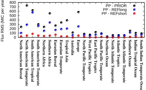
0 100 200 300 400 500 600 700 800

North American Boreal North American Temperate South American Tropical South American Temperate Northern Africa Southern Africa Eurasian Boreal Eurasian Temperate Tropical Asia Australia Europe North Pacific Temperate West Pacific Tropics East Pacific Tropics South Pacific Temperate Northern Ocean North Atlantic Temperate Atlantic Tropics South Atlantic Temperate Southern Ocean Indian Tropical Ocean South Indian Temperate Ocean

Flux RMS (MtC per year)

PP - PRIOR PP - REFlong PP - REFshort

Fig. 3. RMS differences for annual CO₂fluxes between the PP in-version and its prior for the period 1979–2010 (black, PP-PRIOR), between the 1979–2010 PP inversion and the 1979–2010 reference inversion for the same period (blue, PP-REFlong) and between the 1979–2010 PP inversion and the 1979–1992 reference inversion for 1979–1991 (red, PP-REFshort). The world is split into the 22 TransCom3 regions.

NOAA (ftp://ftp.cmdl.noaa.gov/ccg/co2/trends/co2 gr gl.txt accessed 6 September 2012) better than the reference in-version: the root-mean-square difference (RMS) of the mis-fit over the 32 yr is 0.19 ppm yr−1 for the former, while it reaches 0.88 ppm yr−1for the latter. To understand the bet-ter performance of the inversion that uses the simplified sys-tem, the reference inversion is repeated for a shorter period: 1979–1992. In this case, the RMS misfit of the reference in-version with the NOAA data goes down to 0.21 ppm yr−1_,

while the PP misfit is slightly larger (0.22 ppm yr−1_{) for the}

same period. This second reference inversion is also shown in Fig. 2, in standard blue: the curve is well fitted by the PP points, with differences less than 50 Mt C yr−1, even for the year 1990 when the longer reference inversion shows a large spike. From this test and from similar ones varying the length of the inversion window (not shown), we conclude that nu-merical instabilities spoil the reference system for very large inversion windows. The better behaviour of the PP inversion suggests that the small transport sensitivities for very long ranges cause these instabilities.

Figure 3 summarizes the differences between the PP inver-sion and the reference system (run with two inverinver-sion win-dows) at the scale of the year and of the 22 TransCom3 land regions. The RMS is very large (up to 570 Mt C yr−1_in

re-gion South American Tropical) when comparing with the ref-erence system run on the longer window, while it is less than 80 Mt C yr−1when comparing with the reference system run on the shorter window. The misfit with the shorter window system represents about 10 % of the inversion increments.

Figure 4 refines the comparison with the shorter-window reference system by showing the map of the RMS at the weekly grid-point scale. This time scale is chosen because

Fig. 4. RMS differences between the 1979–2010 PP inversion and the reference 1979–1992 inversion when computing the inverted weekly fluxes. The statistics are computed for the 1979–1991 pe-riod.

it is the highest of the inversion system. The RMS is less than 0.08 g C m−2day−1everywhere. Its pattern follows the one of the prior errors (see Fig. 1 of Chevallier et al., 2010). The RMS represents less than 11 % of the flux inversion in-crements on any grid point, excluding those where the incre-ments are negligible.

We have repeated the PP inversion with longer segments. In this test the segments cover 18 months, from July of a given year until December of the following year, with a 6-month overlap from one segment to the next, from July un-til December. In this case, the 1979–1991 fit to the shorter-window reference system is improved by a few percentage points, with the largest relative improvement seen in the ocean basins of the Southern Hemisphere. In terms of annual budgets in the TransCom3 regions, the improvement is less than 20 Mt C yr−1, with most values being a few Mt C yr−1.

6 Discussion and conclusions

More than 10 CO2 monitoring sites have records that span

more than 30 yr and tens of them span more than 20 yr. These archives offer the exceptional opportunity to yield consistent estimations of CO2 surface fluxes over the last

(6)

within variational inversion systems. This approach allows efficient “embarrassingly parallel” workload, i.e. tasks that do not need communicating, within each iteration step. In the case of global inversions, the transport information from one segment to the next one is carried out through a global bias term, while it is not needed for regional inversions. The initial simulation that provides the linearization point before the first iteration as well as the final simulation after the min-imization are not parallelized. At the highest level, the inver-sion manages all segments at once with a single cost func-tion.

For global inversions, the increment bottleneck that we in-troduce in each segment in the form of this bias term (on 1 October of each year in our illustration) reduces the ac-curacy of the tangent-linear model with an effect that de-pends on the assimilated observations: a dense and precise observation network counterbalances the trend towards ho-mogeneously distributed inversion increments because it bet-ter distinguishes between errors in the recent fluxes and errors from the past. In this context, the test with a sin-gle network (the NOAA global cooperative air sampling network), while tens of other sites are available (available at: http://ds.data.jma.go.jp/gmd/wdcgg/), provides an upper bound on the method precision. The effect of the increment bottleneck is also mitigated by the overlap period from one segment to the next that plays the role of a spin-up time. In this study, we have tested our approach with a 3-month over-lap. For a 14 yr inversion window, we have shown that the simplification degrades the inversion increments at various scales (weekly grid scale and sub-yearly continental) by less than 20 %. For a 32 yr inversion window, the simplification makes the inversion numerically stable, which is not the case for the full system that suffers from round-off errors. Lastly, the 32 yr inversion does not take more time to run than for a 15-month inversion (i.e. days rather than months), while still processing the three decades consistently.

Qualitatively, the effect of the transport truncation is bal-anced by the limited robustness of transport models for long ranges. At the global scale, this limitation was clearly seen in the validation of the interhemispheric exchange times simu-lated by a pool of models, even though the precision was shown to have improved compared to older models (Patra et al., 2011). We argue that performing long inversions is important despite transport weaknesses because long inver-sions ensure both the statistical consistency and the physical consistency of the inferred long-term CO2budgets. Indeed,

a sequential filter (e.g. Peters et al., 2007) can either conserve mass throughout the inversion cycles or account for the un-certainty of the past cycles, but cannot do both. Furthermore, long inversions benefit from the long temporal structures of the prior errors (Chevallier et al., 2006), thereby propagating observation information well beyond measurement time in a way that is complementary to transport. This second prop-erty is particularly interesting for regional inversions when

high-resolution flux estimates are sought while the network is sparse at the scale of interest.

For regional (i.e. domain-limited) inversions, the informa-tion about the global growth rate is carried by the atmo-spheric lateral boundary conditions around the inversion do-main. In this case, the bias term disappears from Eq. (2): for a given segment, our method neglects the direct influence of increments of the initial conditions of this segment. The spin-up period (i.e. the between-segment overlap period) damps this effect that becomes negligible when the spin-up period is long enough. An adequate spin-up period mainly depends on the domain latitude range and on the speed of the zonal flow in the domain.

To further improve the inversion speed, additional levels of parallelism can be found in two ways. First, parallel com-puting can be introduced within each segment, in addition to between-segment parallelism. This hybrid parallel strat-egy would fit high-performance computing systems that are usually made of clusters of shared memory nodes. Second, advantage can be taken from ensembles of perturbed inver-sions because they accelerate convergence when performed together (Desroziers and Berre, 2012), while yielding rig-orous inversion uncertainty computation (Chevallier et al., 2007). The parallelization of such ensembles is straightfor-ward because the ensemble members do not communicate.

Among Bayesian systems, the variational ones are the fittest to deal with large inversion problems. The opportu-nities for parallelism that we see in the case of global and re-gional CO2atmospheric inversions reinforce their

attractive-ness in the context of high-performance cluster computing. Our approach also applies when the atmospheric inversion infers parameters of flux process models, like in variational carbon cycle data assimilation systems (Rayner et al., 2005), rather than just the fluxes. We have focused here on CO2

be-cause our method exploits its passive transport in the global atmosphere. It can also be applied for reactive species like methane, nitrogen and chlorofluorocarbons within regional inversions. For global inversions of these species, the distant past cannot be summarized by a constant bias: in this case, Eq. (2) has to be adapted by assigning a lifetime to the global offset.

Acknowledgements. This work was performed using HPC

(7)

Edited by: J. Annan

The publication of this article is financed by CNRS-INSU.

References

Bocquet, M.: Grid resolution dependence in the reconstruction of an atmospheric tracer source, Nonlin. Processes Geophys., 12, 219–233, doi:10.5194/npg-12-219-2005, 2005.

Broquet, G., Chevallier, F., Rayner, P., Aulagnier, C., Pison, I., Ra-monet, M., Schmidt, M., Vermeulen, A., and Ciais, P.: European CO2 biogenic flux inversion at mesoscale from continuous in

situ mixing ratio measurements, J. Geophys. Res, 116, D23303, doi:10.1029/2011JD016202, 2011.

Bruhwiler, L. M. P., Michalak, A. M., Peters, W., Baker, D. F., and Tans, P.: An improved Kalman Smoother for atmospheric inver-sions, Atmos. Chem. Phys., 5, 2691–2702, doi:10.5194/acp-5-2691-2005, 2005.

Chevallier, F., Fisher, M., Peylin, P., Serrar, S., Bousquet, P., Br´eon, F.-M., Ch´edin, A., and Ciais, P.: Inferring CO₂ sources and sinks from satellite observations: method and application to TOVS data, J. Geophys. Res., 110, D24309, doi:10.1029/2005JD006390, 2005.

Chevallier, F., Viovy, N., Reichstein, M., and Ciais, P.: On the assignment of prior errors in Bayesian inversions of CO2 surface fluxes, Geophys. Res. Lett., 33, L13802,

doi:10.1029/2006GL026496, 2006.

Chevallier, F., Br´eon, F.-M., and Rayner, P. J.: The contribu-tion of the Orbiting Carbon Observatory to the estimacontribu-tion of CO2 sources and sinks: theoretical study in a variational

data assimilation framework, J. Geophys. Res., 112, D09307, doi:10.1029/2006JD007375, 2007.

Chevallier, F., Wang, T., Ciais, P., Maignan, F., Bocquet, M., Arain, A., Cescatti, A., Chen, J.-Q., Dolman, H., Law, B. E., Margolis, H. A., Montagni, L., and Moors, E. J.: What eddy-covariance flux measurements tell us about prior errors in CO₂ -flux inversion schemes, Global Biogeochem. Cy., 26, GB1021, doi:10.1029/2010GB003974, 2012.

Chevallier, F., Ciais, P., Conway, T. J., Aalto, T., Anderson, B. E., Bousquet, P., Brunke, E. G., Ciattaglia, L., Esaki, Y., Fr¨ohlich, M., Gomez, A. J., Gomez-Pelaez, A. J., Haszpra, L., Krummel, P., Langenfelds, R., Leuenberger, M., Machida, T., Maignan, F., Matsueda, H., Morgu´ı, J. A., Mukai, H., Nakazawa, T., Peylin, P., Ramonet, M., Rivier, L., Sawa, Y., Schmidt, M., Steele, P., Vay, S. A., Vermeulen, A. T., Wofsy, S., and Worthy, D.: CO₂ surface fluxes at grid point scale estimated from a global 21-year reanalysis of atmospheric measurements, J. Geophys. Res., 115, D21307, doi:10.1029/2010JD013887, 2010.

Conway, T. J., Lang, P. M., and Masarie, K. A.: Atmospheric Car-bon Dioxide Dry Air Mole Fractions from the NOAA ESRL Carbon Cycle Cooperative Global Air Sampling Network, 1968– 2010, Version: 2011-06-21, available at: ftp://ftp.cmdl.noaa.gov/ ccg/co2/flask/event/ (last access: 5 November 2011), 2011.

Desroziers, G. and Berre, L.: Accelerating and paralleliz-ing minimizations in ensemble and deterministic variational assimilations, Q. J. Roy. Meteor. Soc., 138, 1599–1610, doi:10.1002/qj.1886, 2012.

Feng, L., Palmer, P. I., B¨osch, H., and Dance, S.: Estimating surface CO2fluxes from space-borne CO2dry air mole fraction

obser-vations using an ensemble Kalman Filter, Atmos. Chem. Phys., 9, 2619–2633, doi:10.5194/acp-9-2619-2009, 2009.

Fisher, M.: Minimization algorithms for variational data assimila-tion, in: Seminar on Recent Developments in Numerical Methods for Atmospheric Modelling, ECMWF, Reading, 7–11 September 1998, available at: http://www.ecmwf.int/publications/library/ ecpublications/ pdf/seminar/1998/seminar1998 fisher.pdf (last access: 8 January 2013), 1998.

Fisher, M., Tremolet, Y., Auvinen, H., Tan, D., and Poli, P.: Weak-Constraint and Long Window 4DVAR, ECMWF Technical Memorandum No. 655, available at: http://www.ecmwf.int/ publications/library/ecpublications/ pdf/tm/601-700/tm655.pdf (last access: 8 January 2013), 2011.

Gurney, K. R. and Eckels, W. J.: Regional trends in terrestrial car-bon exchange and their seasonal signatures, Tellus B, 63, 328– 339, doi:10.1111/j.1600-0889.2011.00534.x, 2011.

Gurney, K. R., Law, R. M., Denning, A. S., Rayner, P. J., Baker, D., Bousquet, P., Bruhwiler, L., Chen, Y. H., Ciais, P., Fan, S., Fung, I. Y., Gloor, M., Heimann, M., Higuchi, K., John, J., Maki, T., Maksyutov, S., Masarie, K., Peylin, P., Prather, M., Pak, B. C., Randerson, J., Sarmiento, J., Taguchi, S., Takahashi, T., and Yuen, C. W.: Towards robust regional estimates of CO₂sources and sinks using atmospheric transport models, Nature, 415, 626– 630, 2002.

Hamrud, M.: Report from IFS Scalability Project, ECMWF Tech-nical Memorandum No. 616, available at: http://www.ecmwf.int/ publications/library/ecpublications/ pdf/tm/601-700/tm616.pdf (last access: 8 January 2013), 2010.

Hourdin, F., Musat, I., Bony, S., Braconnot, P., Codron, F., Dufresne, J.-L., Fairhead, L., Filiberti, M.-A., Friedlingstein, P., Grandpeix, J.-Y., Krinner, G., and Levan, P.: The LMDZ4 general circulation model: climate performance and sensitivity to parametrized physics with emphasis on tropical convection, Clim. Dynam., 27, 787–813, doi:10.1007/s00382-006-0158-0, 2006.

Kaminski, T., Rayner, P. J., Heimann, M., and Enting, I. G.: On ag-gregation errors in atmospheric transport inversions, J. Geophys. Res., 106, 4703–4715, 2001.

Krinner, G., Viovy, N., de Noblet-Ducoudr´e, N., Og´ee, J., Polcher, J., Friedlingstein, P., Ciais, P., Sitch, S., and Pren-tice, I. C.: A dynamic global vegetation model for studies of the coupled atmosphere-biosphere system, Global Biogeochem. Cy., 19, GB1015, doi:10.1029/2003GB002199, 2005.

Lauvaux, T., Gioli, B., Sarrat, C., Rayner, P. J., Ciais, P., Chevallier, F., Noilhan, J., Miglietta, F., Brunet, Y., Ceschia, E., Dolman, H., Elbers, J. A., Gerbig, C., Hutjes, R., Jarosz, N., Legain, D., and Uliasz, M.: Bridging the gap between atmospheric concen-trations and local ecosystem measurements, Geophys. Res. Lett., 36, L19809, doi:10.1029/2009GL039574, 2009.

(8)

L., Palmer, P. I., Prinn, R. G., Rigby, M., Saito, R., and Wilson, C.: TransCom model simulations of CH4 and related species:

linking transport, surface flux and chemical loss with CH₄ vari-ability in the troposphere and lower stratosphere, Atmos. Chem. Phys., 11, 12813–12837, doi:10.5194/acp-11-12813-2011, 2011. Peters, W., Miller, J. B., Whitaker, J., Denning, A. S., Hirsch, A., Krol, M. C., Zupanski, D., Bruhwiler, L., and Tans, P. P.: An en-semble data assimilation system to estimate CO2surface fluxes

from atmospheric trace gas observations, J. Geophys. Res., 110, D24304, doi:10.1029/2005JD006157, 2005.

Peters, W., Jacobson, A. R., Sweeney, C., Andrews, A. E., Conway, T. J., Masarie, K., Miller, J. B., Bruhwiler, L. M. P., Petron, G., Hirsch, A. I., Worthy, D. E. J., van der Werf, G. R., Randerson, J. T., Wennberg, P. O., Krol, M. C., and Tans, P. P.: An atmospheric perspective on North American carbon dioxide exchange: carbon tracker, P. Natl. Acad. Sci. USA, 48, 18925–18930, 2007. Rayner, P. J., Scholze, M., Knorr, W., Kaminski, T., Giering, R.,

and Widmann, H.: Two decades of terrestrial carbon fluxes from a carbon cycle data assimilation system (CCDAS), Global Bio-geochem. Cy., 19, GB2026, doi:10.1029/2004GB002254, 2005. R¨odenbeck, C.: Estimating CO2 sources and sinks from

at-mospheric mixing ratio measurements using a global inverse of atmospheric transport, Technical Reports, Max-Planck-Institut f¨ur Biogeochemie 6, avilaable at: http://www.bgc-jena.mpg.de/mpg/websiteBiogeochemie/ Publikationen/Technical Reports/tech report6.pdf (last access: 10 February 2011), 2005.

Takahashi, T., Sutherland, S. C., Wanninkhof, R., Sweeney, C., Feely, R. A., Hales, B., Friederich, G., Chavez, F., Watson, A., Bakker, D. C. E., Schuster, U., Metzl, N., Yoshikawa-Inoue, H., Ishii, M., Midorikawa, T., Sabine, C., Hoppema, M., Olaf-sson, J., Arnarson, T. S., Tilbrook, B., Johannessen, T., Olsen, A., Bellerby, R., De Baar, H. J. W., Nojiri, Y., Wong, C. S., Delille, B., and Bates, N. R.: Climatological mean and decadal changes in surface ocean pCO2, and net sea-air CO2 flux

over the global oceans, Deep-Sea Res. Pt. II, 56, 554–577, doi:10.1016/j.dsr2.2008.12.009, 2009.

Thompson, R. L., Gerbig, C., and R¨odenbeck, C.: A Bayesian inver-sion estimate of N₂O emissions for western and central Europe and the assessment of aggregation errors, Atmos. Chem. Phys., 11, 3443–3458, doi:10.5194/acp-11-3443-2011, 2011.

van der Werf, G. R., Randerson, J. T., Giglio, L., Collatz, G. J., Mu, M., Kasibhatla, P. S., Morton, D. C., DeFries, R. S., Jin, Y., and van Leeuwen, T. T.: Global fire emissions and the contribution of deforestation, savanna, forest, agricultural, and peat fires (1997– 2009), Atmos. Chem. Phys., 10, 11707–11735, doi:10.5194/acp-10-11707-2010, 2010.