www.geosci-model-dev.net/5/1/2012/ doi:10.5194/gmd-5-1-2012
© Author(s) 2012. CC Attribution 3.0 License.
Geoscientific
Model Development
Partial Derivative Fitted Taylor Expansion: an efficient method for
calculating gas/liquid equilibria in atmospheric aerosol particles –
Part 2: Organic compounds
D. Topping1,2, D. Lowe2, and G. McFiggans2
1National Centre of Atmospheric Science, Univ. of Manchester, Manchester, M13 9PL, UK
2Centre for Atmospheric Sciences, School of Earth, Atmospheric and Environmental Sciences, Univ. of Manchester,
Manchester, M13 9PL, UK
Correspondence to: D. Topping ([email protected])
Received: 8 June 2011 – Published in Geosci. Model Dev. Discuss.: 2 August 2011 Revised: 30 November 2011 – Accepted: 16 December 2011 – Published: 4 January 2012
Abstract. A flexible mixing rule is presented which al-lows the calculation of activity coefficients of organic com-pounds in a multi-component aqueous solution. Based on the same fitting methodology as a previously published inorganic model (Partial Differential Fitted Taylor series Expansion; PD-FiTE), organic PD-FiTE treats interactions between bi-nary pairs of solutes with polynomials of varying order. The numerical framework of organic PD-FiTE is not based on empirical observations of activity coefficient variation, rather a simple application of a Taylor Series expansion. Using 13 example compounds extracted from a recent sensitivity study, the framework is benchmarked against the UNIFAC model. For 1000 randomly derived concentration ranges and 10 relative humidities between 10 and 99 %, the average de-viation in predicted activity coefficients was calculated to be 3.8 %. Whilst compound specific deviations are present, the median and inter-quartile values across all relative humidity range always fell within±20 % of the UNIFAC value. Com-parisons were made with the UNIFAC model by assuming interactions between solutes can be set to zero within PD-FiTE. In this case, deviations in activity coefficients as low as−40 % and as high as +70 % were found. Both the fully coupled and uncoupled organic PD-FiTE are up to a factor of
≈12 and≈66 times more efficient than calling the UNIFAC model using the same water content, and≈310 and≈1800 times more efficient than an iterative model using UNIFAC. The use of PD-FiTE within a dynamical framework is pre-sented, demonstrating the potential inaccuracy of prescrib-ing fixed negative or positive deviations from ideality when modelling the evolving chemical composition of aerosol par-ticles.
1 Introduction and rationale
Gas to particle partitioning, driven by a difference in equi-librium and partial pressures, is a key process that dictates the evolving chemical composition of atmospheric aerosol particles, thus their environmental impacts. The equilibrium vapour pressure above a solution is given by:
Pi=Poγixi (1)
where Pi is the equilibrium vapour pressure, Po the pure
component vapour pressure,γi the activity coefficient in
so-lution andxi the mole fraction of componenti in solution.
Sensitivity to choice of predictive technique for calculating Po, in terms of aerosol mass and properties, has recently
been reviewed by McFiggans et al. (2010) and Topping et al. (2011). In this paper we use the technique for calculating Porecommended by Barley et al. (2009).
In a previous publication, a new hybrid reduced complex-ity ionic mixing rule for calculating γi and hence,
2 D. Topping et al.: Partial Derivative Fitted Taylor Expansion
and interaction terms derived by fitting this framework to a more complex benchmark model (UNIFAC). This fitting methodology is the same methodology applied to inorganic PD-FiTE, despite the different approach used in defining the model terms and concentration scales, hence we use the same acronym here.
Activity coefficients account for interactions taking place in solution. Numerous model are available for both inor-ganic, organic and mixed inorganic-organic solutions. Un-fortunately these models are far too expensive for inclusion in large scale models (Zaveri et al., 2005; Topping et al., 2009). As inorganic and organic activity coefficient frame-works have different theoretical constructs it is difficult to build reduced complexity frameworks which are equally ap-plicable to both systems (Zuend et al., 2011). Following inor-ganic PD-FiTE, in this paper we use the same Taylor Series expansion methodology to develop a model for organic so-lutes in aqueous solutions via an appropriate representation of multi-component concentrations and interactions. Assess-ing the accuracy of both the inorganic and organic versions of PD-FiTE to mixed inorganic-organic aqueous systems will form the focus of a future study, using the revised AIOMFAC model as a benchmark (Zuend et al., 2011).
2 Reduced complexity activity coefficient framework
The numerical basis for the inorganic PD-FiTE is a simple Taylor series expansion involving only the first order term:
lnγi(xj00,x
00
k,...RH)=lnγio(RH)+ N
X
j6=i ∂lnγi
∂xj00
!
(RH)xj00 (2) where lnγi(RH) is the activity coefficient of component i in the mixture as a function of relative humidity (RH), lnγio(RH)the binary activity coefficient of componenti in water at a given RH,xi00the equivalent mole fraction of com-ponenti. As described by Topping et al. (2009), the interac-tion terms implicitly account for any effects of partial disso-ciation of the HSO4-ion. Since the dissociation of organics
cannot be modelled with any certainty (Clegg and Seinfeld, 2006), only interactions between undissociated molecules are considered. For the organic model, interactions are re-stricted to binary pairs of solutes, thus reducing computa-tional cost. The activity coefficient function then takes on the following general form:
γ=F ( N
X
i=1
ci N
X
j6=i
cj) (3)
WhereN represents the total number of solutes, ci andcj
represent a specific concentration scale for componentsiand j. Models such as UNIQUAC (Abrams et al., 1975) and the Wilson (Wilson, 1964) equations also treat binary interac-tions, the mixture represented by the sum of these pairs. In the residual and combinatorial expressions of the UNIQUAC
model, binary pairs are coupled using absolute mole fractions weighted according to molecular surface area and volume pa-rameters:
8i= rixi
Pm j=1rjxj
(4)
θi= qixi
Pm
j=1qjxj
(5)
wheremrepresents the total number of compounds,riandqi
are the surface area and volume parameters for componentsi with associated mole fractionxi. In organic PD-FiTE, choice
of concentration scale can be chosen according to the limit-ing requirements of the numerical framework. The numeri-cal framework of organic PD-FiTE is not based on empirinumeri-cal observations of activity coefficient variation, rather the same parameter fitting methodology is used as the inorganic work,as detailed in Sect. 3. The ability of this new frame-work to replicate activity coefficients for various concentra-tions is given in Sect. 4 where the UNIFAC model is used as a benchmark. As with inorganic PD-FiTE, for a one com-ponent system (i.e. one organic solute in water), the activity coefficient of the solute must equal the binary activity coef-ficient in water. This represents the first term in the Taylor series expansion:
lnfi(xj=o,xk=o,...)=lnfio (6)
where we use the symbolf to represent activity coefficients of organic solutes. As inorganic PD-FiTE was based on the empirical observation that the logarithm of solute activity co-efficients varies roughly linearly with water activity, thus RH for a bulk solution, Eq. (6) would be written explicitly as a function of RH were we able to use the same basis. As mentioned previously, this framework does not use the same empirical basis. For the inorganic model, the range of com-pounds defining the composition space was relatively small and, using the PD-FiTE fitting methodology, the variation in water activity of the whole system was well constrained. For the organic model, it is likely that the compounds se-lection will change depending on the application, thus sys-tems studied. Whilst the water activity scale could be used, given the fitting methodology optimizes interaction terms, as new compounds are introduced every model parameter would have to be refit. To mitigate this problem, a differ-ent concdiffer-entration scale is chosen . In Eq. (2), the expression x refers to equivalent mole fractions. In the first instance, the Taylor Series expression used for organic PD-FiTE is ex-pressed using mole fractions of components in the multicom-ponent mixture (including water). For the organic model, bi-nary activity coefficients and interaction are expressed as a function of water mole fraction. The reason for this is two-fold. Firstly, this will aid development of coupled inorganic-organic approaches in the future. Whilst interaction terms between inorganic and organic components are not presented here, the effect of dilution by the water associated with the
inorganic fraction can be used to effect the organic solute ac-tivity coefficients in a semi-coupled approach. Secondly, the combination of data from binary systems assumes the solvent to be water. This allows future expansion without the need to run a thermodynamic model to derive fits as a function of RH for each binary pair. It is possible that multiple phases exist in aerosol particles in the atmosphere. However, solving this problem is extremely challenging even for ternary systems (Zuend et al., 2011) and currently cannot be generalised to complex mixtures of multiple organic and inorganic solutes. In the absence of treatment of phase separation or mixed sol-vent system, taking water as the solsol-vent Eq. (6) becomes: lnfi(xj=o,xk=o,...xw)=lnfio(xw) (7)
and the generic Taylor series expansion is written as: lnfi(xj,xk,...xw)=lnfio(xw)+
N
X
j6=i
∂lnf
i ∂xj
(xw)xj (8)
The reliance on data from binary systems is an important feature of any flexible organic activity framework. Whilst the inorganic fraction of aerosol particles is restricted to small range of compounds, the number of organic compounds act-ing as potential condensates can be very large. With this in mind, the form of the expression encapsulated within the summation can now be chosen. Taking a hypothetical ternary system of organic compounds “A” and “B”, starting with a bi-nary solution of component “A” in water, as component “B” is added, the deviation in activity coefficientfAhas to be
ac-counted for using an appropriate concentration scale. Equa-tion (8) can be re-written as:
lnfA(xB,xw)=lnfAo(xw)+
N
X
j6=i
∂lnf
A
∂xB
(xw)xB (9)
To ensure correct limiting behaviour, the difference be-tween the binary activity coefficient lnfAo(xw)and ternary
activity coefficient lnfA(xB,xw)can be expressed a function
of dry solute mole fractions. As the dry mole fraction of so-lute “B” approaches zero, the term∂lnfA
∂xB
xw
converges to zero. Therefore, for a specific mole fraction of water, Eq. (9) is re-written as:
lnfA(xB0,xw=c)=lnfAo(xw=c)+
∂lnf
A
∂xB0
xw=c
xB0 (10) where xB0 is the dry mole fraction of solute “B”. As “B” tends to zero, the activity coefficient of “A” converges to the binary activity coefficient at a specific concentration of wa-ter. Parameters in inorganic PD-FiTE were optimised using the ADDEM thermodynamic model (Topping et al., 2005). The same parameter optimisation approach is used here. The term ∂lnfA
∂xB0
xw=c
xB0 is re-written as a specific function of xB0:
∂lnf
A
∂xB0
xw=c
xB0 =(β(F (xB0))xw=c) (11)
whereβ now represents a scaling factor in lnfA, at a
spe-cific concentration of water, as the dry solute mole fraction of “B” changes. Whilst a simple scaling factor that varies lin-early withxB0 could be used, the order of polynomial chosen (e.g. linear, quadratic, cubic, etc) is based on accuracy of fit as compared to UNIFAC predictions as described in Sect. 4. Equation (11) is not complete and variability of∂lnfA
∂xB0
as a function ofxwis required. As the concentration of
compo-nent “A” approaches zero, the magnitude of the dependence ofβ(F (xB0))on the concentration of water increases. There-fore we introduce another variable to Eq. (11):
∂lnf
A
∂xB0
=(β(F (xB0))xw)∗(α(F (xw))xA→0) (12)
where(α(F (xw))xA→0)represents the variation of
∂lnf
A ∂x0
B
as a function of water mole fraction as “A” approaches zero, and (βx0
B) represents the scaling of (α(F (xw))xA→0) as a
function ofxB0.
We can now write the generalised expression for lnfAas:
lnfA(xB0,x
0
C,x
0
D,...xw)=lnfAo(xw)+
N
X
i6=A
(βi,A(xi0)xw)(αi,A(xw)xA→0) (13)
Where the variables encapsulated within the summation can be expressed as:
αB,A(xwxA→0)=
C(0)∗xwo+C(1)∗xwo−1..[o=polynomial order] (14) βB,A(xB0)xw=
D(0)∗x0Bo+D(1)∗x0Bo−1..[o=polynomial order] (15) The rationale behind the above framework is best illus-trated using an example. Two compounds were randomly selected within the UNIFAC framework with the following functional groups: (1) CH3×2, CH2×1, OH×1, COOH×1
(compound “A”); (2) CH2×1, COOH×1 (compound “B”).
Figure 1 shows a surface plot of lnfA(xB0,xw)−lnfAo(xw)or
1lnfA as a function ofxB0 andxw. As the “dry” mole
frac-tion of solute “B” tends to zero, the value of1lnfAtends to
zero for all concentrations of water. However, as “A” tends to zero, the variability of1lnfAvaries non-linearly as a
func-tion ofxw, the magnitude increases as “A” decreases.
In any higher order systems, the assumption is made that the behaviour of each binary pair holds in the mixture. How-ever, the use of total mole fractions and dry mole fractions ensures an appropriate dilution effect is captured. Compar-isons between organic PD-FiTE with the UNIFAC model are presented in Sect. 4.
4 D. Topping et al.: Partial Derivative Fitted Taylor Expansion
Fig. 1.Difference in activity coefficient of compound “A” as a function ofx0
Bandxw. The colour-scale
is bound by red (low values) to purple (high values) figure
30
Fig. 1. Difference in activity coefficient of compound “A” as a func-tion ofxB0 andxw. The colour-scale is bound by red (low values) to
purple (high values).
Fig. 2. Difference in activity coefficient of compound 1 as a function ofx0
3andxw. The compound numbers and SMILES strings are listed in Table 1. The colour-scale is bound by red (low values) to purple (high values)
31
Fig. 2. Difference in activity coefficient of compound 1 as a func-tion ofx03andxw. The compound numbers and SMILES strings are
listed in Table 1. The colour-scale is bound by red (low values) to purple (high values).
3 Parameter fitting 3.1 Activity coefficients
Using the same methodology described by Topping et al. (2009), the interaction terms in the model are optimised based on fitting to a more complex scheme, the UNIFAC model (Fredenslund et al., 1975). Parameters (βB,A(xB0)xw) and (αB,A(xw)xA→0) are expressed using
polynomials as a function ofxB0 andxw respectively. The
required level of complexity, or order of the polynomials, are dictated by setting the tolerance on two independent statistical variables, automating the whole process. The order of fitting to both parameters is important. First, the polynomials for(αB,A(xw)xA→0)are determined by setting
the dry mole fraction of “A”, xA0 to a negligible amount
Fig. 3. Difference in activity coefficient of compound 1 as a function ofx0
4andxw. The compound numbers and SMILES strings are listed in Table 1. The colour-scale is bound by red (low values) to purple (high values)
32
Fig. 3. Difference in activity coefficient of compound 1 as a func-tion ofx40andxw. The compound numbers and SMILES strings are
listed in Table 1. The colour-scale is bound by red (low values) to purple (high values).
(0.0001). Following this, the mole fraction of water is varied and the xw axes in Fig. 1 is populated. The order of the
polynomial is chosen by selecting the best fit between 1st to 8th order polynomials in the MATLAB software package 7.6.0 (R2008a). For each polynomial fit, the coefficients are derived through initialisation with a random number generator which is run 1000 times, the fitting routine using the Levenberg Marquardt algorithm. The point at which the order of a polynomial meets the criteria for being chosen is defined as: (1) the pairwise linear correlation coefficient between UNIFAC predictions and the polynomial fit is greater than 0.99 or (2) when there is no significant decrease in the sum of the square of the residuals as the degree of polynomial is increased. The cutoff value used for the second criteria was set to 10−4.
Following this, the polynomial for(βB,A(xB0)xw)was
de-rived by choosing a slice from the surface displayed in Fig. 1 as a function ofxB0. The value ofxwchosen to define the
lo-cation of this slice is that which corresponds to the maximum value of(αB,A(xw)xA→0). Subsequent values of1lnfAas a
function ofxB0 are then normalised to this value to give us the scaling factors used to derive(βB,A(x0B)xw).
The order of the polynomial chosen is defined using the same procedure outlined above. Using this approach it is possible to use less computationally expensive polynomials, whilst retaining accuracy, as compared to pre-defined poly-nomial orders for each case (e.g. a 5th order polypoly-nomial for each value of(βB,A(xB0)xw)and(αB,A(xw)xA→0)). For
Fig. 4.
Comparing binary/ternary PD-FiTE and UNIFAC for a random specific testcase. Each subplot
represents a specific RH. Linear correlation coefficients are given in each subplot title. ’Rb’ and ’Rt’
are the correlation coefficients for the binary and ternary model respectively. For this specific example,
the compounds with the largest deviations from the binary model are 3,4,7,8,9 and 10.The compound
numbers and SMILES strings are listed in Table 1 and average percentage deviations in Table 4.
33
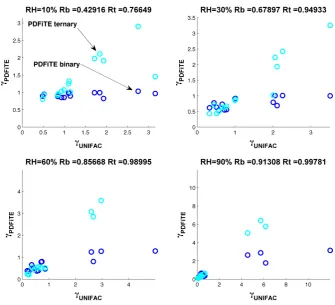
Fig. 4. Comparing binary/ternary PD-FiTE and UNIFAC for a random specific testcase. Each subplot represents a specific RH. Linear correlation coefficients are given in each subplot title. ’Rb’ and ’Rt’ are the correlation coefficients for the binary and ternary model, respectively. For this specific example, the compounds with the largest deviations from the binary model are 3, 4, 7, 8, 9 and 10. The compound numbers and SMILES strings are listed in Table 1 and average percentage deviations in Table 4.
that the direction of1lnfA is at least captured. In applying
the framework to a specific set of compounds in Sect. 4, the automated procedure is used. For binary activity coefficients lnfAo(xw), the same automated procedure is used.
3.2 Calculating water content
For calculating water content, thus mole fractions in solution, the ZSR mixing rule is used (Zdanovskii, 1936). This method has been reviewed extensively in the literature and therefore not analysed here. Using ZSR, the water content associated with each compound at a specific relative humidity is added together to calculate the water content of the mixture:
wt(RH)= N
X
i=1
wi(RH) (16)
where the individual water contents are fit to UNIFAC for a range of water activities (0 to 0.99). The mole fraction of water associated with each solutexwi(RH)is fit to the
UNI-FAC model to ensure a well behaved polynomial fit (rather than absolute water content). The water content associated
with each solute can then be calculated using the following expression:
wi(RH)=nixwi(RH)/(1−xwi(RH)) (17)
whereni is the number of moles of solutei.
4 Benchmarking PD-FiTE against UNIFAC
In the following section Eq. (13) is applied to a specific set of compounds and benchmarked against the UNIFAC model.
6 D. Topping et al.: Partial Derivative Fitted Taylor Expansion
Table 1. Compound identification for fitting as presented within the Master Chemical Mechanism (Jenkin et al., 1997).
Compound MCM SMILES C H O N Cl Structure number number
1 3442 OC(=O)C=CC(=O)O 4 4 4 0 0
Table 1.
Compound identification for fitting as presented within the Master Chemical
Mecha-nism (Jenkin et al , 1997).
Compound
MCM
SMILES
C
H
O
N
Cl
Structure
number
number
1
3442
OC(=O)C=CC(=O)O
4
4
4
0
0
2
4823
OCC(C(ON(=O)=O)(C)C)CC(=O)C(O)=O
8
13
7
1
0
3
4610
OOC1(CCC2C(C1C2)(C)C)CO
10
18
3
0
0
4
4855
CC1(C)C(CON(=O)=O)CC1C(O)=O
8
13
5
1
0
5
2635
C(O)C1C(C(C(C)=O)(C1)OO)(C)C
9
16
4
0
0
6
4834
OOC1(CC(CO)C1(C)C)C(=O)O
8
14
5
0
0
7
4608
CC1(C2CCC(CO)(C1C2)ON(=O)=O)C
10
17
4
1
0
8
4435
OOC1C2(OOC(C2O)(C=C1C)CC)C
10
16
5
0
0
9
4830
CC1(C)C(CC1CC(=O)OON(=O)=O)C(=O)O
9
13
7
1
0
10
2605
C12C(C(CC(C1(C)OO)O)C2)(C)C
10
18
3
0
0
11
2617
CC(C(CC(CO)C(C)(ON(=O)=O)C)=O)=O
9
15
6
1
0
12
5482
OC(C(CO)OO)(C)C
5
12
4
0
0
13
3447
OC(=O)C(=O)C(O)C(=O)O
4
4
6
0
0
22
2 4823 OCC(C(ON(=O)=O)(C)C)CC(=O)C(O)=O 8 13 7 1 0
Table 1.
Compound identification for fitting as presented within the Master Chemical
Mecha-nism (Jenkin et al , 1997).
Compound MCM SMILES C H O N Cl Structure
number number
1 3442 OC(=O)C=CC(=O)O 4 4 4 0 0
2 4823 OCC(C(ON(=O)=O)(C)C)CC(=O)C(O)=O 8 13 7 1 0
3 4610 OOC1(CCC2C(C1C2)(C)C)CO 10 18 3 0 0
4 4855 CC1(C)C(CON(=O)=O)CC1C(O)=O 8 13 5 1 0
5 2635 C(O)C1C(C(C(C)=O)(C1)OO)(C)C 9 16 4 0 0
6 4834 OOC1(CC(CO)C1(C)C)C(=O)O 8 14 5 0 0
7 4608 CC1(C2CCC(CO)(C1C2)ON(=O)=O)C 10 17 4 1 0
8 4435 OOC1C2(OOC(C2O)(C=C1C)CC)C 10 16 5 0 0
9 4830 CC1(C)C(CC1CC(=O)OON(=O)=O)C(=O)O 9 13 7 1 0
10 2605 C12C(C(CC(C1(C)OO)O)C2)(C)C 10 18 3 0 0
11 2617 CC(C(CC(CO)C(C)(ON(=O)=O)C)=O)=O 9 15 6 1 0
12 5482 OC(C(CO)OO)(C)C 5 12 4 0 0
13 3447 OC(=O)C(=O)C(O)C(=O)O 4 4 6 0 0
22
3 4610 OOC1(CCC2C(C1C2)(C)C)CO 10 18 3 0 0
Table 1.
Compound identification for fitting as presented within the Master Chemical
Mecha-nism (Jenkin et al , 1997).
Compound
MCM
SMILES
C
H
O
N
Cl
Structure
number
number
1
3442
OC(=O)C=CC(=O)O
4
4
4
0
0
2
4823
OCC(C(ON(=O)=O)(C)C)CC(=O)C(O)=O
8
13
7
1
0
3
4610
OOC1(CCC2C(C1C2)(C)C)CO
10
18
3
0
0
4
4855
CC1(C)C(CON(=O)=O)CC1C(O)=O
8
13
5
1
0
5
2635
C(O)C1C(C(C(C)=O)(C1)OO)(C)C
9
16
4
0
0
6
4834
OOC1(CC(CO)C1(C)C)C(=O)O
8
14
5
0
0
7
4608
CC1(C2CCC(CO)(C1C2)ON(=O)=O)C
10
17
4
1
0
8
4435
OOC1C2(OOC(C2O)(C=C1C)CC)C
10
16
5
0
0
9
4830
CC1(C)C(CC1CC(=O)OON(=O)=O)C(=O)O
9
13
7
1
0
10
2605
C12C(C(CC(C1(C)OO)O)C2)(C)C
10
18
3
0
0
11
2617
CC(C(CC(CO)C(C)(ON(=O)=O)C)=O)=O
9
15
6
1
0
12
5482
OC(C(CO)OO)(C)C
5
12
4
0
0
13
3447
OC(=O)C(=O)C(O)C(=O)O
4
4
6
0
0
22
4 4855 CC1(C)C(CON(=O)=O)CC1C(O)=O 8 13 5 1 0
Table 1.
Compound identification for fitting as presented within the Master Chemical
Mecha-nism (Jenkin et al , 1997).
Compound MCM SMILES C H O N Cl Structure
number number
1 3442 OC(=O)C=CC(=O)O 4 4 4 0 0
2 4823 OCC(C(ON(=O)=O)(C)C)CC(=O)C(O)=O 8 13 7 1 0
3 4610 OOC1(CCC2C(C1C2)(C)C)CO 10 18 3 0 0
4 4855 CC1(C)C(CON(=O)=O)CC1C(O)=O 8 13 5 1 0
5 2635 C(O)C1C(C(C(C)=O)(C1)OO)(C)C 9 16 4 0 0
6 4834 OOC1(CC(CO)C1(C)C)C(=O)O 8 14 5 0 0
7 4608 CC1(C2CCC(CO)(C1C2)ON(=O)=O)C 10 17 4 1 0
8 4435 OOC1C2(OOC(C2O)(C=C1C)CC)C 10 16 5 0 0
9 4830 CC1(C)C(CC1CC(=O)OON(=O)=O)C(=O)O 9 13 7 1 0
10 2605 C12C(C(CC(C1(C)OO)O)C2)(C)C 10 18 3 0 0
11 2617 CC(C(CC(CO)C(C)(ON(=O)=O)C)=O)=O 9 15 6 1 0
12 5482 OC(C(CO)OO)(C)C 5 12 4 0 0
13 3447 OC(=O)C(=O)C(O)C(=O)O 4 4 6 0 0
22
5 2635 C(O)C1C(C(C(C)=O)(C1)OO)(C)C 9 16 4 0 0
Table 1.
Compound identification for fitting as presented within the Master Chemical
Mecha-nism (Jenkin et al , 1997).
Compound
MCM
SMILES
C
H
O
N
Cl
Structure
number
number
1
3442
OC(=O)C=CC(=O)O
4
4
4
0
0
2
4823
OCC(C(ON(=O)=O)(C)C)CC(=O)C(O)=O
8
13
7
1
0
3
4610
OOC1(CCC2C(C1C2)(C)C)CO
10
18
3
0
0
4
4855
CC1(C)C(CON(=O)=O)CC1C(O)=O
8
13
5
1
0
5
2635
C(O)C1C(C(C(C)=O)(C1)OO)(C)C
9
16
4
0
0
6
4834
OOC1(CC(CO)C1(C)C)C(=O)O
8
14
5
0
0
7
4608
CC1(C2CCC(CO)(C1C2)ON(=O)=O)C
10
17
4
1
0
8
4435
OOC1C2(OOC(C2O)(C=C1C)CC)C
10
16
5
0
0
9
4830
CC1(C)C(CC1CC(=O)OON(=O)=O)C(=O)O
9
13
7
1
0
10
2605
C12C(C(CC(C1(C)OO)O)C2)(C)C
10
18
3
0
0
11
2617
CC(C(CC(CO)C(C)(ON(=O)=O)C)=O)=O
9
15
6
1
0
12
5482
OC(C(CO)OO)(C)C
5
12
4
0
0
13
3447
OC(=O)C(=O)C(O)C(=O)O
4
4
6
0
0
22
6 4834 OOC1(CC(CO)C1(C)C)C(=O)O 8 14 5 0 0
Table 1.
Compound identification for fitting as presented within the Master Chemical
Mecha-nism (Jenkin et al , 1997).
Compound
MCM
SMILES
C
H
O
N
Cl
Structure
number
number
1
3442
OC(=O)C=CC(=O)O
4
4
4
0
0
2
4823
OCC(C(ON(=O)=O)(C)C)CC(=O)C(O)=O
8
13
7
1
0
3
4610
OOC1(CCC2C(C1C2)(C)C)CO
10
18
3
0
0
4
4855
CC1(C)C(CON(=O)=O)CC1C(O)=O
8
13
5
1
0
5
2635
C(O)C1C(C(C(C)=O)(C1)OO)(C)C
9
16
4
0
0
6
4834
OOC1(CC(CO)C1(C)C)C(=O)O
8
14
5
0
0
7
4608
CC1(C2CCC(CO)(C1C2)ON(=O)=O)C
10
17
4
1
0
8
4435
OOC1C2(OOC(C2O)(C=C1C)CC)C
10
16
5
0
0
9
4830
CC1(C)C(CC1CC(=O)OON(=O)=O)C(=O)O
9
13
7
1
0
10
2605
C12C(C(CC(C1(C)OO)O)C2)(C)C
10
18
3
0
0
11
2617
CC(C(CC(CO)C(C)(ON(=O)=O)C)=O)=O
9
15
6
1
0
12
5482
OC(C(CO)OO)(C)C
5
12
4
0
0
13
3447
OC(=O)C(=O)C(O)C(=O)O
4
4
6
0
0
22
7 4608 CC1(C2CCC(CO)(C1C2)ON(=O)=O)C 10 17 4 1 0
Table 1.
Compound identification for fitting as presented within the Master Chemical
Mecha-nism (Jenkin et al , 1997).
Compound
MCM
SMILES
C
H
O
N
Cl
Structure
number
number
1
3442
OC(=O)C=CC(=O)O
4
4
4
0
0
2
4823
OCC(C(ON(=O)=O)(C)C)CC(=O)C(O)=O
8
13
7
1
0
3
4610
OOC1(CCC2C(C1C2)(C)C)CO
10
18
3
0
0
4
4855
CC1(C)C(CON(=O)=O)CC1C(O)=O
8
13
5
1
0
5
2635
C(O)C1C(C(C(C)=O)(C1)OO)(C)C
9
16
4
0
0
6
4834
OOC1(CC(CO)C1(C)C)C(=O)O
8
14
5
0
0
7
4608
CC1(C2CCC(CO)(C1C2)ON(=O)=O)C
10
17
4
1
0
8
4435
OOC1C2(OOC(C2O)(C=C1C)CC)C
10
16
5
0
0
9
4830
CC1(C)C(CC1CC(=O)OON(=O)=O)C(=O)O
9
13
7
1
0
10
2605
C12C(C(CC(C1(C)OO)O)C2)(C)C
10
18
3
0
0
11
2617
CC(C(CC(CO)C(C)(ON(=O)=O)C)=O)=O
9
15
6
1
0
12
5482
OC(C(CO)OO)(C)C
5
12
4
0
0
13
3447
OC(=O)C(=O)C(O)C(=O)O
4
4
6
0
0
22
8 4435 OOC1C2(OOC(C2O)(C=C1C)CC)C 10 16 5 0 0
Table 1.
Compound identification for fitting as presented within the Master Chemical
Mecha-nism (Jenkin et al , 1997).
Compound
MCM
SMILES
C
H
O
N
Cl
Structure
number
number
1
3442
OC(=O)C=CC(=O)O
4
4
4
0
0
2
4823
OCC(C(ON(=O)=O)(C)C)CC(=O)C(O)=O
8
13
7
1
0
3
4610
OOC1(CCC2C(C1C2)(C)C)CO
10
18
3
0
0
4
4855
CC1(C)C(CON(=O)=O)CC1C(O)=O
8
13
5
1
0
5
2635
C(O)C1C(C(C(C)=O)(C1)OO)(C)C
9
16
4
0
0
6
4834
OOC1(CC(CO)C1(C)C)C(=O)O
8
14
5
0
0
7
4608
CC1(C2CCC(CO)(C1C2)ON(=O)=O)C
10
17
4
1
0
8
4435
OOC1C2(OOC(C2O)(C=C1C)CC)C
10
16
5
0
0
9
4830
CC1(C)C(CC1CC(=O)OON(=O)=O)C(=O)O
9
13
7
1
0
10
2605
C12C(C(CC(C1(C)OO)O)C2)(C)C
10
18
3
0
0
11
2617
CC(C(CC(CO)C(C)(ON(=O)=O)C)=O)=O
9
15
6
1
0
12
5482
OC(C(CO)OO)(C)C
5
12
4
0
0
13
3447
OC(=O)C(=O)C(O)C(=O)O
4
4
6
0
0
22
9 4830 CC1(C)C(CC1CC(=O)OON(=O)=O)C(=O)O 9 13 7 1 0
Table 1.
Compound identification for fitting as presented within the Master Chemical
Mecha-nism (Jenkin et al , 1997).
Compound MCM SMILES C H O N Cl Structure
number number
1 3442 OC(=O)C=CC(=O)O 4 4 4 0 0
2 4823 OCC(C(ON(=O)=O)(C)C)CC(=O)C(O)=O 8 13 7 1 0
3 4610 OOC1(CCC2C(C1C2)(C)C)CO 10 18 3 0 0
4 4855 CC1(C)C(CON(=O)=O)CC1C(O)=O 8 13 5 1 0
5 2635 C(O)C1C(C(C(C)=O)(C1)OO)(C)C 9 16 4 0 0
6 4834 OOC1(CC(CO)C1(C)C)C(=O)O 8 14 5 0 0
7 4608 CC1(C2CCC(CO)(C1C2)ON(=O)=O)C 10 17 4 1 0
8 4435 OOC1C2(OOC(C2O)(C=C1C)CC)C 10 16 5 0 0
9 4830 CC1(C)C(CC1CC(=O)OON(=O)=O)C(=O)O 9 13 7 1 0
10 2605 C12C(C(CC(C1(C)OO)O)C2)(C)C 10 18 3 0 0
11 2617 CC(C(CC(CO)C(C)(ON(=O)=O)C)=O)=O 9 15 6 1 0
12 5482 OC(C(CO)OO)(C)C 5 12 4 0 0
13 3447 OC(=O)C(=O)C(O)C(=O)O 4 4 6 0 0
22
10 2605 C12C(C(CC(C1(C)OO)O)C2)(C)C 10 18 3 0 0
Table 1.
Compound identification for fitting as presented within the Master Chemical
Mecha-nism (Jenkin et al , 1997).
Compound
MCM
SMILES
C
H
O
N
Cl
Structure
number
number
1
3442
OC(=O)C=CC(=O)O
4
4
4
0
0
2
4823
OCC(C(ON(=O)=O)(C)C)CC(=O)C(O)=O
8
13
7
1
0
3
4610
OOC1(CCC2C(C1C2)(C)C)CO
10
18
3
0
0
4
4855
CC1(C)C(CON(=O)=O)CC1C(O)=O
8
13
5
1
0
5
2635
C(O)C1C(C(C(C)=O)(C1)OO)(C)C
9
16
4
0
0
6
4834
OOC1(CC(CO)C1(C)C)C(=O)O
8
14
5
0
0
7
4608
CC1(C2CCC(CO)(C1C2)ON(=O)=O)C
10
17
4
1
0
8
4435
OOC1C2(OOC(C2O)(C=C1C)CC)C
10
16
5
0
0
9
4830
CC1(C)C(CC1CC(=O)OON(=O)=O)C(=O)O
9
13
7
1
0
10
2605
C12C(C(CC(C1(C)OO)O)C2)(C)C
10
18
3
0
0
11
2617
CC(C(CC(CO)C(C)(ON(=O)=O)C)=O)=O
9
15
6
1
0
12
5482
OC(C(CO)OO)(C)C
5
12
4
0
0
13
3447
OC(=O)C(=O)C(O)C(=O)O
4
4
6
0
0
22
11 2617 CC(C(CC(CO)C(C)(ON(=O)=O)C)=O)=O 9 15 6 1 0
Table 1.
Compound identification for fitting as presented within the Master Chemical
Mecha-nism (Jenkin et al , 1997).
Compound
MCM
SMILES
C
H
O
N
Cl
Structure
number
number
1
3442
OC(=O)C=CC(=O)O
4
4
4
0
0
2
4823
OCC(C(ON(=O)=O)(C)C)CC(=O)C(O)=O
8
13
7
1
0
3
4610
OOC1(CCC2C(C1C2)(C)C)CO
10
18
3
0
0
4
4855
CC1(C)C(CON(=O)=O)CC1C(O)=O
8
13
5
1
0
5
2635
C(O)C1C(C(C(C)=O)(C1)OO)(C)C
9
16
4
0
0
6
4834
OOC1(CC(CO)C1(C)C)C(=O)O
8
14
5
0
0
7
4608
CC1(C2CCC(CO)(C1C2)ON(=O)=O)C
10
17
4
1
0
8
4435
OOC1C2(OOC(C2O)(C=C1C)CC)C
10
16
5
0
0
9
4830
CC1(C)C(CC1CC(=O)OON(=O)=O)C(=O)O
9
13
7
1
0
10
2605
C12C(C(CC(C1(C)OO)O)C2)(C)C
10
18
3
0
0
11
2617
CC(C(CC(CO)C(C)(ON(=O)=O)C)=O)=O
9
15
6
1
0
12
5482
OC(C(CO)OO)(C)C
5
12
4
0
0
13
3447
OC(=O)C(=O)C(O)C(=O)O
4
4
6
0
0
22
12 5482 OC(C(CO)OO)(C)C 5 12 4 0 0
Table 1.
Compound identification for fitting as presented within the Master Chemical
Mecha-nism (Jenkin et al , 1997).
Compound
MCM
SMILES
C
H
O
N
Cl
Structure
number
number
1
3442
OC(=O)C=CC(=O)O
4
4
4
0
0
2
4823
OCC(C(ON(=O)=O)(C)C)CC(=O)C(O)=O
8
13
7
1
0
3
4610
OOC1(CCC2C(C1C2)(C)C)CO
10
18
3
0
0
4
4855
CC1(C)C(CON(=O)=O)CC1C(O)=O
8
13
5
1
0
5
2635
C(O)C1C(C(C(C)=O)(C1)OO)(C)C
9
16
4
0
0
6
4834
OOC1(CC(CO)C1(C)C)C(=O)O
8
14
5
0
0
7
4608
CC1(C2CCC(CO)(C1C2)ON(=O)=O)C
10
17
4
1
0
8
4435
OOC1C2(OOC(C2O)(C=C1C)CC)C
10
16
5
0
0
9
4830
CC1(C)C(CC1CC(=O)OON(=O)=O)C(=O)O
9
13
7
1
0
10
2605
C12C(C(CC(C1(C)OO)O)C2)(C)C
10
18
3
0
0
11
2617
CC(C(CC(CO)C(C)(ON(=O)=O)C)=O)=O
9
15
6
1
0
12
5482
OC(C(CO)OO)(C)C
5
12
4
0
0
13
3447
OC(=O)C(=O)C(O)C(=O)O
4
4
6
0
0
22
13 3447 OC(=O)C(=O)C(O)C(=O)O 4 4 6 0 0
Table 1.
Compound identification for fitting as presented within the Master Chemical
Mecha-nism (Jenkin et al , 1997).
Compound
MCM
SMILES
C
H
O
N
Cl
Structure
number
number
1
3442
OC(=O)C=CC(=O)O
4
4
4
0
0
2
4823
OCC(C(ON(=O)=O)(C)C)CC(=O)C(O)=O
8
13
7
1
0
3
4610
OOC1(CCC2C(C1C2)(C)C)CO
10
18
3
0
0
4
4855
CC1(C)C(CON(=O)=O)CC1C(O)=O
8
13
5
1
0
5
2635
C(O)C1C(C(C(C)=O)(C1)OO)(C)C
9
16
4
0
0
6
4834
OOC1(CC(CO)C1(C)C)C(=O)O
8
14
5
0
0
7
4608
CC1(C2CCC(CO)(C1C2)ON(=O)=O)C
10
17
4
1
0
8
4435
OOC1C2(OOC(C2O)(C=C1C)CC)C
10
16
5
0
0
9
4830
CC1(C)C(CC1CC(=O)OON(=O)=O)C(=O)O
9
13
7
1
0
10
2605
C12C(C(CC(C1(C)OO)O)C2)(C)C
10
18
3
0
0
11
2617
CC(C(CC(CO)C(C)(ON(=O)=O)C)=O)=O
9
15
6
1
0
12
5482
OC(C(CO)OO)(C)C
5
12
4
0
0
13
3447
OC(=O)C(=O)C(O)C(=O)O
4
4
6
0
0
22
Table 2. Polynomials for binary activity coefficient: lnγio=A(0)∗xworder+A(1)∗xworder−1..[order=polynomialorder].
Number A(0) A(1) A(2) A(3) A(4) A(5) A(6)
1 −0.680844 −0.030474 0.013327
2 18.342261 −36.865487 26.174686 −8.565417 0.962597 −0.027869
3 150.945646 −382.149648 369.674775 −168.512416 34.234823 −3.179822 0.070701 4 283.084624 −718.473072 695.657994 −313.71093 63.550996 −6.148153 0.136931 5 76.065039 −149.766159 109.111489 −33.639646 3.971213 −0.115294
6 203.421677 −520.253952 506.342017 −230.816455 46.618829 −4.442629 0.099128 7 74.2173 −154.863304 114.946223 −39.048428 4.340771 −0.127665
8 130.648433 −266.724081 199.936973 −63.122582 6.558979 −0.196416
9 274.762453 −697.581434 675.811261 −304.968978 61.546109 −5.961812 0.132819 10 85.387073 −168.601696 122.96918 −37.927336 4.48584 −0.130329
11 279.043008 −700.756563 677.314976 −307.85783 66.107566 −5.767339 0.128072 12 185.68401 −472.462525 458.242015 −208.337606 43.242955 −4.003782 0.089179 13 7.850520 −12.415950 2.418568 −0.159090
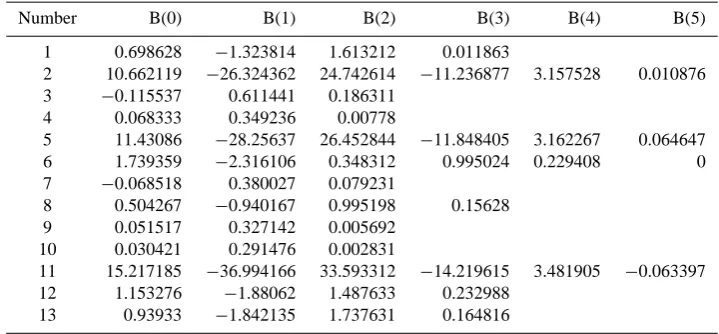
Table 3. Polynomials for water content: logxwio =B(0)∗(RH/100)order+B(1)∗(RH/100)order−1.
Number B(0) B(1) B(2) B(3) B(4) B(5)
1 0.698628 −1.323814 1.613212 0.011863
2 10.662119 −26.324362 24.742614 −11.236877 3.157528 0.010876 3 −0.115537 0.611441 0.186311
4 0.068333 0.349236 0.00778
5 11.43086 −28.25637 26.452844 −11.848405 3.162267 0.064647 6 1.739359 −2.316106 0.348312 0.995024 0.229408 0 7 −0.068518 0.380027 0.079231
8 0.504267 −0.940167 0.995198 0.15628 9 0.051517 0.327142 0.005692
10 0.030421 0.291476 0.002831
11 15.217185 −36.994166 33.593312 −14.219615 3.481905 −0.063397 12 1.153276 −1.88062 1.487633 0.232988
13 0.93933 −1.842135 1.737631 0.164816
order to extract a subset of compounds to be used as an ex-ample on the applicability of PD-FiTE. The resulting com-pounds defined in that study are listed in Table 1 along with their SMILES string, compound identification number as fined within the MCM and chemical structure. Specific de-tails regarding the selection methodology are presented in Appendix A. The simplified molecular input line entry spec-ification or SMILES is a specspec-ification for unambiguously describing the structure of chemical molecules using short ASCII strings. Each compound SMILES representation was translated into appropriate UNIFAC functional groups using the PyBel toolbox (O’Boyle et al., 2008) and a complete set of SMARTS to represent the Hansen et al. (1991) UNI-FAC matrix. For a more detailed discussion of SMILES and SMARTS, the reader is referred to the Daylight Chemical Information systems webpage (www.daylight.com). To il-lustrate the use of Eq. (13), the polynomials used to calculate
the binary activity coefficient and water content of each com-pound are listed in Tables 2 and 3 respectively. An example subset of the polynomials used to calculate interactions be-tween each solute pair are given in Appendix B.
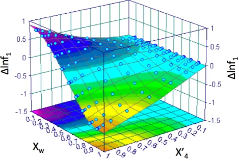
To illustrate the behaviour of compounds listed in Table 1, Figs. 2 and 3 show surface plots of 1lnf1 as a function
of xB0 andxw for two separate ternary mixtures with
com-pounds “3” and “4”. As the ‘dry’ mole fraction of solute “B”, or compounds “3” and “4” approach zero, the value of 1lnf1tends to zero for all concentrations of water. Whilst
the presence of solute “3” always decreases lnf1relative to
a binary solution of only solute “1” in water, the presence of solute “4” can increase or decrease lnf1depending on the
concentration of water. As described in Sect. 2, each sur-face is used to fit the interaction parameters (βB,A(xB0)xw)
8 D. Topping et al.: Partial Derivative Fitted Taylor Expansion
Fig. 5.Ratio of activity coefficients predicted by PD-FiTE to UNIFAC as a function of RH. Blue boxes correspond to PD-FiTE binary and cyan to PD-FiTE ternary. Using the MATLAB R2008a software package, the box represents the upper/lower quartile range with the median highlighted inbetween. The whiskers represent values within the 10 and 90 percentile boundaries, outliers representing any values greater than 1.5 times the inter-quartile range.
34
Fig. 5. Ratio of activity coefficients predicted by PD-FiTE to UNI-FAC as a function of RH. Blue boxes correspond to PD-FiTE bi-nary and cyan to PD-FiTE terbi-nary. Using the MATLAB R2008a software package, the box represents the upper/lower quartile range with the median highlighted inbetween. The whiskers represent val-ues within the 10 and 90 percentile boundaries, outliers representing any values greater than 1.5 times the inter-quartile range.
Fig. 6.Cumulative CPU time for each 100’th call of each activity coefficient model. Two variations of the UNIFAC model correspond to using the same water content as calculated in PD-FiTE (using ZSR “WZSR” and using an iterative solver).
35
Fig. 6. Cumulative CPU time for each 100’th call of each activity coefficient model. Two variations of the UNIFAC model correspond to using the same water content as calculated in PD-FiTE (using ZSR “WZSR” and using an iterative solver).
To benchmark PD-FiTE, the original UNIFAC model is used with the updated parameters of Peng et al. (2001). The version of PD-FiTE defined by Eq. (13) is hereafter referred to as “PD-FiTE-ternary” as it account for interactions be-tween binary pairs of solutes in water. Comparisons are also made with PD-FiTE assuming that all solute-solute interac-tions can be set to zero such that the summation term in Eq. (13) is not used. This variant shall hereafter be referred to “PD-FiTE-binary” as it represents individual solutes in
wa-Table 4. Average percentage deviations between PD-FiTE and UNIFAC. Statistics averaged across 100 random initializations at ten relative humidities (10, 20, 30, 40, 50, 60, 70, 80, 90, 99 %), providing 1000 datapoints.
Compound Binary Ternary
number PD-FiTE PD-FiTE
1 19.45440718 −14.30912809 2 2.673215656 6.101359896 3 −47.36864158 −3.702870758 4 −53.60107768 18.70554837 5 52.25168852 21.06698518 6 20.46580233 −2.837865435 7 −73.25882432 2.225730891 8 −44.90977498 −7.648612446 9 −58.64378672 21.61434862 10 −77.72342066 1.873670474 11 41.95350378 39.9819442 12 15.37105714 14.5210335 13 −33.46446243 −27.46755099
Overall −16.12413131 3.807365426
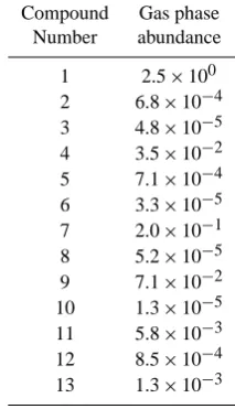
Table 5. Mixing ratios (ppt) of each compound used within the dynamical simulation.
Compound Gas phase Number abundance
1 2.5×100 2 6.8×10⁻⁴ 3 4.8×10⁻⁵ 4 3.5×10⁻² 5 7.1×10⁻⁴ 6 3.3×10⁻⁵ 7 2.0×10⁻¹ 8 5.2×10⁻⁵ 9 7.1×10⁻² 10 1.3×10⁻⁵ 11 5.8×10⁻³ 12 8.5×10⁻⁴ 13 1.3×10⁻³
ter. An analysis of the accuracy of both approaches is impor-tant since “PD-FiTE-binary” is less computational expensive than “PD-FiTE-ternary” as discussed in Sect. 5. Pre-defining concentrations of inorganic compounds to benchmark the model for a range of typical environments is relatively easy, (Zaveri et al., 2005). For organic compounds, however, this is less clear. For this reason, in this study, concentrations of each compound in Table 1 were randomly generated using uniformly distributed pseudorandom numbers in the MAT-LAB software package 7.6.0 (R2008a). In total, 100 relative
Table 6. Polynomials representing interactions between solute “A” (compound “1” in Table 1) and solutes “B” (compounds 3, 4 and 5 in Table 1), where “A” tends to zero;(αB,A(xw)xA→0)= C(0)∗
xworder+C(1)∗xworder−1..[order=polynomial order].
Solute “B” C(0) C(1) C(2) C(3) C(4) C(5) C(6) 3 −8.564 15.172 −5.018 0.263 −0.977
4 −19.872 30.857 −10.779 0.996 0.666 5 −19.718 28.945 −12.553 3.13 0.959
Table 7. Polynomials representing interactions between so-lute “A” (compound ’1’ in Table 1) and soso-lutes “B” (com-pounds 3, 4 and 5 in Table 1), for a specific concentration of water as “B” changes; (βB,A(xB0)xw) = D(0)∗x
0
Border+D(1)∗
x0
Border−1..[order=polynomial order].
Solute “B” D(0) D(1) D(2) D(3) D(4) D(5) D(6) 3 1.416 −0.455 0.01
4 0.405 0.593 0.001 5 0.229 0.771 0.0004
concentrations for each compound were derived using the Mersenne Twister algorithm. For each concentration the rel-ative humidity was varied between 10 to 99 %, resulting in a different water content calculated using the ZSR rule. For comparisons with the UNIFAC model the same water con-tent was used. Some overall statistics are discussed before individual compound analysis is given.
Figure 4 displays scatter plots for both the binary and ternary version of PD-FiTE versus UNIFAC for four dif-ferent relative humidities (10, 30, 60 and 90 %). Taking the 10 % RH case, ternary PD-FiTE clearly correlates bet-ter with UNIFAC than binary PD-FiTE, as confirmed by the Pearson squared correlation coefficients (0.96 and 0.40, re-spectively). The performance of binary PD-FiTE decreases as the activity coefficients increase. This is to be expected as the highly non-linear influence of multiple solutes is not captured within the binary framework. As the relative hu-midity increases the correlation coefficient of both variants improves. Figure 5 plots the ratio of predictions from both binary and ternary PD-FiTE as compared to UNIFAC across 100 sets of simulations at 10 different relative humidities. The ternary model is clearly more accurate than the binary variant, with median values always within ±20 % across all relative humidity ranges. Predictions from binary PD-FiTE lie across a much broader distribution with deviations as low as−40 % and as high as +70 % in the inter-quartile range. Table 4 provides average deviations for each indi-vidual compound across all simulations and relative humidi-ties. Whilst some detail provided by Figs. 4 and 5 is lost within the average statistics, average percentage deviations from ternary PD-FiTE are smaller than those from binary PD-FiTE. For example, for compound 7 used in this study,
and listed in Table 4, the percentage deviation on changing from the ternary to the binary model can increase from 2.2 % to−73.3 %. Multiple outliers have influenced the derivation of mean values which should be combined with the distribu-tions presented in Fig. 5. Overall, binary PD-FiTE is statis-tically less accurate than ternary PD-FiTE with total average deviations of−16.12 % and 3.8 %, respectively.
5 Computational performance
Figure 6 displays the cumulative CPU time in seconds after each set of 100 calls to both PD-FiTE (binary and ternary) and UNIFAC for the 100 sets of simulations described in Sect. 4. Whilst a comparison of the number of floating point operations might be advantageous, this is difficult to attribute to an iterative approach using UNIFAC. There are two lines representing UNIFAC: the first represents the use of water contents calculated using the ZSR approach within PD-FiTE, the second represents an iterative solution for both water con-tents and activity coefficients. No code was parallelised for this comparison. All routines were written in the Matlab software package which was run on a windows XP machine (2.66 Ghz Intel dual core, 2GB RAM). In each case, the fixed parameters within the model were saved to memory at the first call. Given the number of permutations in ternary PD-FiTE this significantly reduces run time. The binary version of PD-FiTE is the most efficient method, as to be expected. The order of the polynomials used to represent interactions within the ternary PD-FiTE model are optimised during the fitting process. Therefore it is difficult to directly relate the generic increase in computational cost of the ternary method over the binary method. For the compounds analysed in this study, ternary PD-FiTE is less efficient than the binary vari-ant by a factor of≈6, as indicated in Fig. 6. However, both ternary and binary PD-FiTE are up to a factor of≈12 and
≈66 times more efficient than calling the UNIFAC model using the same water content, and≈310 and ≈1800 times more efficient than an iterative model using UNIFAC.
6 Dynamical testcases
10 D. Topping et al.: Partial Derivative Fitted Taylor Expansion
0 6 12 18 24
0.10 1.00
Dry Radius [
µ
m]
Time [Hours] (a)
PP − VP [atm]
−1 −0.5 0 0.5 1 1.5 x 10⁻¹⁰
0 0.5 1 1.5 2 2.5
x 10−10
PP [atm]
0 6 12 18 24
0.10 1.00
Dry Radius [
µ
m]
Time [Hours] (c)
PP − VP [atm]
−1 −0.5 0 0.5 1 1.5 x 10⁻¹⁰
0 0.5 1 1.5 2 2.5
x 10−10
PP [atm]
0 6 12 18 24
0.10 1.00
Time [hours] (b)
Dry Radius [
µ
m]
Dry Mole Fraction
0 0.05 0.1 0.15 0.2 0.25 0.3
0 6 12 18 24
0.10 1.00
Time [hours] (d)
Dry Radius [
µ
m]
Dry Mole Fraction
0 0.05 0.1 0.15 0.2 0.25 0.3
Fig. 7.
Evolving condensed phase abundance and gas phase concentration for compound “8” as a
func-tion of time, assuming ideality (
a
and
b
) and using PD-FiTE (
c
and
d
). Panels
(a)
and
(c)
show the
size-resolved differences between vapour pressure (VP) over aerosol particles and the gas-phase partial
pressure (PP) (red indicates higher partial pressures; blue indicates higher vapor pressures), as well as
the temporal variation in the partial pressure of compound “8” (black line). Panels
(b)
and
(d)
show the
size-resolved dry mole fractions of compound “8” within the condensed-phase.
36
Fig. 7. Evolving condensed phase abundance and gas phase concentration for compound “8” as a function of time, assuming ideality (a and b) and using PD-FiTE (c and d). Panels (a) and (c) show the size-resolved differences between vapour pressure (VP) over aerosol particles and the gas-phase partial pressure (PP) (red indicates higher partial pressures; blue indicates higher vapor pressures), as well as the temporal variation in the partial pressure of compound “8” (black line). Panels (b) and (d) show the size-resolved dry mole fractions of compound “8” within the condensed-phase.
0 6 12 18 24
0.10 1.00
Dry Radius [
µ
m]
Time [Hours] (a)
PP − VP [atm]
−2 0 2 4 x 10⁻¹²
0 1 2 3 4 5 6x 10
−12
PP [atm]
0 6 12 18 24
0.10 1.00
Dry Radius [
µ
m]
Time [Hours] (c)
PP − VP [atm]
−2 0 2 4 x 10⁻¹²
0 1 2 3 4 5 6x 10
−12
PP [atm]
0 6 12 18 24
0.10 1.00
Time [hours] (b)
Dry Radius [
µ
m]
Dry Mole Fraction
0 0.02 0.04 0.06
0 6 12 18 24
0.10 1.00
Time [hours] (d)
Dry Radius [
µ
m]
Dry Mole Fraction
0 0.02 0.04 0.06
Fig. 8.
Evolving condensed phase abundance and gas phase concentration for compound “12” as a
function of time, assuming ideality (
a
and
b
) and using PD-FiTE (
c
and
d
). Panels
(a)
and
(c)
show the
size-resolved differences between vapour pressure (VP) over aerosol particles and the gas-phase partial
pressure (PP) (red indicates higher partial pressures; blue indicates higher vapor pressures), as well as
the temporal variation in the partial pressure of compound “12” (black line). Panels
(b)
and
(d)
show the
size-resolved dry mole fractions of compound “12” within the condensed-phase.
37
Fig. 8. Evolving condensed phase abundance and gas phase concentration for compound “12” as a function of time, assuming ideality (a and b) and using PD-FiTE (c and d). Panels (a) and (c) show the size-resolved differences between vapour pressure (VP) over aerosol particles and the gas-phase partial pressure (PP) (red indicates higher partial pressures; blue indicates higher vapor pressures), as well as the temporal variation in the partial pressure of compound “12” (black line). Panels (b) and (d) show the size-resolved dry mole fractions of compound “12” within the condensed-phase.
semivolatile species to the condensed-phase does not deplete the gas-phase mixing ratios. The maximum mixing ratios, taken from an online box model simulation using the MCM are given in Table 5 .
The condensed phase consists of 1 aerosol distribution, comprised of 64 individual size-sections. Particle growth across the size-sections within each mode is dealt with us-ing the Movus-ing Centre method. The aerosol distribution is initialised with 2 log-normal modes, each with a represen-tative involatile core (hereafter referred to as compounds 14 and 15, used to represent primary and heavily oygenated or-ganic aerosol). The first log-normal mode has a mode radius of 0.2 µm, width of 1.7, and total particle number of 10 cm−air3; the second has a mode radius of 0.02 µm, width of 2.0, and total particle number of 2000 cm−air3. The total dry aerosol mass is 3.5 µg m−air3, temperature is 285.15 K, and relative hu-midity is 75 %. These compounds are used purely as a way to initialise an existing aerosol distribution, the functionality of compound 15, was assumed to be that reported for fulvic acid (Topping et al., 2005).
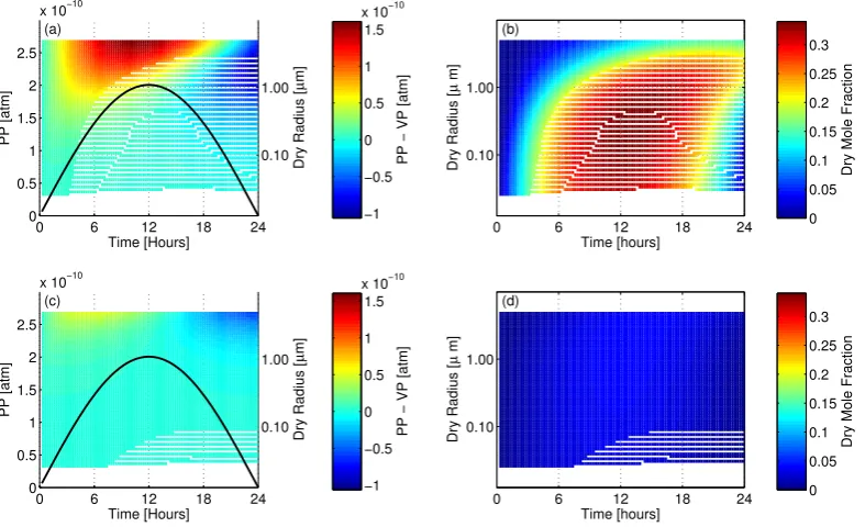
The testcase was run twice: (1) assuming ideality, and (2) using PD-FiTE to calculate activity coefficients over 24 h (model time). Semivolatile partitioning is driven by the difference between atmospheric partial pressure and vapour pressure of the species over the condensed-phase. The size-resolved vapour pressure differences for each of the 13 semi-volatile species, as well as the size-resolved dry mole frac-tions for each of the 15 condensed-phase species are pro-vided as supplementary material; for brevity, however, we will only examine the behaviour of two compounds: Com-pound “8” (Fig. 7); and ComCom-pound “12” (Fig. 8) which ex-hibit positive and negative deviations from ideality respec-tively. In Figs. 7 and 8 the coloured surface plots show the differences between partial pressure and vapour pressure across the size ranges of the two aerosol modes for each semivolatile gas species (plotted as the difference in atmo-spheres; red indicates higher partial pressures; blue indicates higher vapour pressures). The black lines show the abso-lute gas phase concentrations of each semivolatile gas species during the model run.
Compound “12” is the dominate condensed-phase semi-volatile species in this example (Compound “1” has a higher partial pressure, but is also more volatile, and so does not contribute as much to the condensed phase), with a dry mole fraction close to 0.35 at 12 h across the majority of the aerosol distribution in the ideal testcase (Fig. 7b). Pressure differences are highest over the largest particles (Fig. 7a); with diffusion controlled condensation rates these large par-ticles never achieve equilibrium with the gas-phase. The in-troduction of non-ideality greatly increases the volatility of compound “12”, decreasing the vapour pressures over all particles sizes (Fig. 7c) and reducing the dry mole fraction maxima to≈0.1 (Fig. 7d).
Compound “5” has a lower abundance than compound “12”, but is also less volatile, and so reaches a dry mole fraction of ≈0.025 at 12 h in the ideal testcase (Fig. 8b). The lower volatility causes greater pressure differences over more of the particle size distribution (Fig. 8a), leading to the mole fraction in the smaller particles to continue increasing (leading to greater composition gradients across the particle size-range). Non-ideality greatly decreases the volatility of compound “12”, increasing the vapour pressure differences (Fig. 8c), which leads to an increase in the dry mole fraction maxima to≈0.065 at 12 h (Fig. 8d).
This simulation demonstrates the ability of PD-FiTE to be used stably in dynamical simulations of multicomponent aerosol evolution in a changing gaseous environment. Whilst it is difficult to derive generalised conclusions to one exam-ple dynamical testcase, it is interesting to observe both the positive and negative deviations from ideality resulting from interactions taking place in solution. This was also found by Barley et al. (2011) who performed a much broader as-sessment of the sensitivity to non-ideality within an equilib-rium framework. This demonstrates the potential inaccuracy in prescribing fixed negative or positive deviations from ide-ality when modelling the evolving chemical composition of aerosol particles.
7 Conclusions and future work
A simple, flexible mixing rule is presented which allows the calculation of activity coefficients, thus equilibrium vapour pressures, of organic condensates above a multi-component aqueous solution. Based on the same fitting methodology as a previously published inorganic model (PD-FiTE), organic PD-FiTE treats interactions between binary pairs of solutes with variable sets of polynomials. Using 13 compounds ex-tracted from an example gas phase degradation mechanism, the framework is benchmarked against the UNIFAC model. For 1000 randomly derived concentration ranges and 10 rel-ative humidities between 10 and 99 %, the average deviation was calculated to be 3.8 %. Whilst compound specific devi-ations did vary, the median and inter-quartile values across all relative humidity range always fell within±20 %. Com-parisons were also made with organic PD-FiTE by assuming interactions between solutes can be set to zero. Predictions from this approach lie across a much broader distribution with deviations as low as−40 % and as high as +70 % in the inter-quartile range, with an average deviation of−16.1 %. The computational cost of both variants was compared to the use of UNIFAC for the same amounts of water. Both the fully coupled and uncoupled organic PD-FiTE are up to a factor of
12 D. Topping et al.: Partial Derivative Fitted Taylor Expansion
Whilst improvements in the accuracy of UNIFAC have been made and widely implemented, it is difficult to prescribe complete confidence to predictions from multi-component solutions across a broad range of concentrations. Focused laboratory studies are required to validate predictions from these mixed systems. However, the flexible nature of organic PD-FiTE allows direct inclusion of any improvements in the predictive skill of the UNIFAC framework.
The inorganic and organic versions of PD-FiTE currently remain uncoupled. Since a revised version of the AIMO-FAC framework has recently been published (Zuend et al., 2011), a thorough comparison of inorganic and organic PD-FiTE with this model will form the focus of future work. The use of organic PD-FiTE within a dynamical framework is demonstrated, highlighting the potential inaccuracy in pre-scribing fixed negative or positive deviations from ideality when modelling the evolving aerosol composition.
Appendix A
Reduction methodology used to select the 13 example compoundsused to benchmark PD-FiTE
In Barley et al. (2011), Master Chemical Mechanism (Jenkin et al. (1997)MCM) simulations were conducted in such a way as to cover a wide range of emission scenarios rep-resenting high anthropogenic and low biogenic sources as well as high biogenic and low anthropogenic sources. sions representing average UK National Atmospheric Emis-sions Inventory (NAEI) emission totals for the year 2001 (3740 ktonnes CO, 1130 ktonnes SO2, 1680 ktonnes NOx,
and 1510 ktonnes speciated VOCs with 1330 ktonnes being anthropogenic AVOCs) were continuously emitted into the box throughout the model run. Further emission scenar-ios were simulated by independently multiplying the anthro-pogenic VOCs (AVOCs), biogenic VOCs (BVOC) and NOx
component of the base case emissions by factors of 0.01, 0.1, 10, 100 and 1000 to give a total of 216 emission scenarios covering a swing of 6 orders of magnitude in the emitted concentrations. With such an extreme range in emissions, ten scenarios gave unrealistically high ozone mixing ratios (>300 ppb). These scenarios were sensibly removed. For each emission scenario the partitioning calculation was con-ducted at a number of temperature, RH and involatile core mass, giving a set of 24 cases:
– Temperature (K): 273.15, 283.15, 293.15 and 303.15 – RH (%): 0, 50 and 90
– Mass of involatile core (µg m−3): 0.5 and 3.0
Where the involatile core is assumed to interact ideally with all components and is assigned a molar mass of 320 g mole−1, based on the analysis of water soluble organic compounds (WSOC) reported by Reemtsma et al. (2006).
The top 13 contributing compounds to SOA using the Nanoolal VP (Nannoolal et al., 2008) and Tb (Nannoolal et al., 2004) method were found by averaging across all sce-narios and all conditions, results displayed in Table 1.
Appendix B
Example set of polynomials used to calculate solute interactions in PD-FiTE
Described in the main body of text, the activity coefficient of an organic solute is represented by the expression:
lnfA(xB0,x
0
C,x
0
D,...xw)=lnfAo(xw)+
N
X
i6=A
(βi,A(xi0)xw)(αi,A(xw)xA→0) (B1)
As an example, the polynomials for(αB,A(xw)xA→0),
deter-mined by setting the dry mole fraction of “A”,xA0 to a negli-gible amount (0.0001) are given for compound combinations 3-1, 4-1, 5-1 in Table 6. The polynomials for(βB,A(xB0)xw)
for the same solute combinations are also displayed in Ta-ble 7. As described in the main body of text,(βB,A(xB0)xw)
represents a scaling factor for(αB,A(xw)xA→0)as the ratio
of solute “A” to “B” changes. The Matlab implementation of the PD-FiTE model described in this paper is also provided as supplementary material with examples given for polyno-mial coefficients. Written in MATLAB R2008a, only the core toolboxes are called. Converting from Matlab to Fortran is relatively straightforward, with a Fortran version available on request. It will be possible to develop bespoke versions of PD-FiTE using an online interface which is currently under development. This will provide multiple language versions of the PD-FiTE model on request.
Supplementary material related to this article is available online at:
http://www.geosci-model-dev.net/5/1/2012/ gmd-5-1-2012-supplement.pdf.
Acknowledgements. DOT was supported by UK National Centre
for Atmospheric Science (NCAS) funding. DL was supported by the RONOCO (ROle of Nightime chemistry in controlling the Oxidising Capacity of the AtmOsphere. NE/F004664/1) and VO-CALS (VAMOS Ocean-Cloud-Atmosphere-Land. NE/F019874/1) projects. Additional support was provided by the NERC funded informatics project, grant number NE/H002588/1.
Edited by: R. Sander
![Table 7.Polynomials representing interactions between so-xlute “A” (compound ’1’ in Table 1) and solutes “B” (com-pounds 3, 4 and 5 in Table 1), for a specific concentration ofwater as “B” changes; (βB,A(x′B)xw) = D(0) ∗ x′Border + D(1) ∗′Border−1..[order = polynomial order].](https://thumb-us.123doks.com/thumbv2/123dok_us/9111001.1903746/9.595.56.276.263.307/polynomials-representing-interactions-compound-specic-concentration-border-polynomial.webp)