SProt: sphere-based protein structure similarity algorithm

(1)

P R O C E E D I N G S

Open Access

SProt: sphere-based protein structure similarity

algorithm

Jakub Galgonek

*

, David Hoksza

*

, Tomá

š

Skopal

From

International Workshop on Computational Proteomics

Hong Kong, China. 18-21 December 2010

Abstract

Background:Similarity search in protein databases is one of the most essential issues in computational proteomics. With the growing number of experimentally resolved protein structures, the focus shifted from sequences to structures. The area of structure similarity forms a big challenge since even no standard definition of optimal structure similarity exists in the field.

Results:We propose a protein structure similarity measure called SProt. SProt concentrates on high-quality

modeling of local similarity in the process of feature extraction. SProt’s features are based on spherical spatial

neighborhood of amino acids where similarity can be well-defined. On top of the partial local similarities, global measure assessing similarity to a pair of protein structures is built. Finally, indexing is applied making the search process by an order of magnitude faster.

Conclusions:The proposed method outperforms other methods in classification accuracy on SCOP superfamily and fold level, while it is at least comparable to the best existing solutions in terms of precision-recall or quality of alignment.

Background

The biological function of a protein is consequence of its spatial conformation rather than of ordering of its amino acids (protein sequence). Thus, the protein struc-ture is closer to the function than the sequence, there-fore there was an enormous effort spent on protein structure research. Moreover, the biological motivation for protein structure similarity stems from the thesis that proteins having similar structures also share similar function. Hence, it is very useful to have tools for mea-suring protein structure similarity in order to be able to identify similar protein structures from a database of protein structures with already known function.

Most of the protein structure similarity measures are based on comparisons of positions of amino acids in the space. For this purpose, amino acids are represented as coordinates of theira-carbon (and sometimesb-carbon)

atoms. The protein structure similarity assessment usually comprises two steps. In the first one, which we call alignment search, an amino acid inter-protein pair-ing is established. The second step, which we call super-position search, includes superposition optimizing the selected similarity function. This function usually aggre-gates values based on spatial (euclidean) distances of the paired amino acids after the superposition.

Although it has been shown that if the optimal solu-tion is required, the above defined measuring of struc-ture similarity is NP-hard [1] (non-deterministic polynomial-time), each step of the problem can be solved in polynomial time using the result of the other step. If we know the alignment, there exist methods how to obtain superposition optimizing given similarity

formula in polynomial time, e.g., theKabsch algorithm

[2] for root mean square deviation (RMSD). On the other hand, if we are provided with the superposition and the similarity formula in a form of sum, we can use dynamic programming to determine the optimal align-ment with respect to the given superposition. The

* Correspondence: [email protected]; [email protected] Siret Research Group, Faculty of Mathematics and Physics, Charles University in Prague, Malostranské nám. 25, 118 00 Prague, Czech Republic

Full list of author information is available at the end of the article

(2)

dynamic programming has to employ a scoring corre-sponding to the inner part of the sum. If using RMSD, the score ofi-th andj-th amino acids of the superposed proteins is defined as their squared euclidean distance. As the solution of structure similarity consists of steps that depend each on the other, at the beginning we do not know neither the alignment nor the superposition.

We briefly describe the main ideas of some of the state-of-the-art algorithms and also some solutions which outperform the other ones and which we com-pare to our contribution— DALI,ProtDex2, CE, SSAP, MAMMOTH, Vorometric, Vorolign, PPM, db-iTM, BLAST,PSI-BLAST,3D-BLAST.

One of the earliest approaches to protein structure

similarity assessment was DALI, representing the

pro-tein’s structure by a two-dimensional matrix of inter-residual distances [3,4]. Similar protein structures should also share similar distance distribution, thus in the com-parison process the matrices are split into overlapping parts and similar (contact) patterns are stored. These are further extended to obtain the alignment.

Similarly to DALI,ProtDex2 uses intra-residual

dis-tance matrices [5]. However, instead of chaining the contact patterns, ProtDex2 splits them to constant-sized submatrices which, together with their description, are used as index terms for inverted index. Protein struc-tures used as queries are processed in the same way. The inverted index together with subsequent scoring is utilized to identify similar protein structures in the data-base. The query result could be furthermore refined by an arbitrary alignment-based algorithm.

The CEmethod uses the concept of aligned fragment

pairs (AFP) for searching structurally similar portions of the sequences [6]. In particular, a few seeds are chosen and iteratively extended by chaining with other AFPs. Three different measures are taken into account when deciding whether a new AFP should be added to the chain. At the end, a final optimization is performed which results in the best alignment.

TheSSAP method [7] heavily exploits

Smith-Water-man dynamic programming algorithm [8]. Each residue is represented by distances to every other residue. For each pair of amino acids in the compared protein struc-tures a dynamic programming is used with scoring matrix based on the residue distances (local similarity). In the second-level dynamic programming, the matrices are aggregated to obtain the resulting structure align-ment (global similarity).

Another well-known method for comparison of two protein structures is MAMMOTH [9]. MAMMOTH represents each amino acid by its sequence neighbor-hood that is 7 amino acids long (heptapeptide). The unit-vector root mean square for each pair of heptapep-tides is computed and forwarded into the

Smith-Waterman algorithm as a scoring matrix. The output of Smith-Waterman forms an alignment of the two struc-tures. Maximum subset of aligned pairs being spatially close after superposition (based on the alignment) is

taken into account for computing so-calledpercentage

of structural identity(PSI). In the last step, probability of obtaining the given PSI by chance (P-value) is calcu-lated as the final result.

More recently, methods based on Voronoi diagrams

were proposed. TheVorometric method forms contact

strings from the Delaunay tessellation and these are stored in a metric index [10]. For finding similar contact string with the query, edit distance with metric scoring matrix is used. The resulting hits are used as seeds for the consequent step, where a modification of dynamic programming is applied to the hits in order to obtain the alignment.

Vorolign extracts nearest-neighbor sets for each amino acid based on the Voronoi tessellation [11]. There is a similarity of the sets defined, which is further used in dynamic programming for assessing local similarity to a pair of amino acids. The local similarities are used as scores for second-level dynamic programming. The same group of authors introduced later a solution called

PPM[12]. PPM identifies sufficiently similar (core)

blocks which are then used to create a graph of core blocks. That path in the graph is chosen, that minimizes the cost of mutations.

The db-iTMmethod is a recently proposed solution which represents amino acids as a set of concentric cir-cles [13]. Based on their densities and radii, the method

forms feature vectors used in local dynamic

programming.

Last of the structure-based methods presented in this

overview is 3D-BLAST[14]. This method derives

struc-tural alphabet from the-a plot. The structures repre-sented as strings over this alphabet are accessed using the BLAST approach. That takes us to other methods which are purely sequence-based and thus we are able to provide comparison of structure-based approaches

with the sequence-based ones – BLAST[15] and

PSI-BLAST[16]. BLAST is the state-of-the-art tool for simi-larity search in protein sequence databases. It is based on heuristics which noticeably decreases runtime needed for the full Smith-Waterman algorithm [8], which is the optimal measure for assessing similarity to a pair of pro-tein sequences. PSI-BLAST extends the original BLAST algorithm by employment of a position-specific scoring matrix, so that it is more sensitive to weak sequential similarities.

In this work, we propose our own approach to protein structure similarity, called SProt, based on high-quality modeling of local similarity in the process of feature

(3)

spherical spatial neighborhoods of amino acids, because on them the similarity can be well-defined. Along with the proposed similarity measure, we also introduce an access method that reduces the number of applications of the measure and so the real-time cost. The effective-ness and efficiency of the proposed approach is evalu-ated by experiments.

Methods

In contrast to most of the presented algorithms, in our solution we put a lot of emphasis on high-quality mod-eling of local similarities of the amino acids. We believe that representing proteins by various derived features might cause loss of information which is inevitable for quality alignment. In this section we present our solu-tion, calledSProt, which aims to avoid the possible loss-of-information drawback.

SProt fundamentals

As we have already mentioned, determining alignment and superposition of protein structures is a nontrivial problem. However, what holds true for whole protein structures does not have to be valid for small substruc-tures. If we want to align two small parts of two protein backbones, the natural way is to execute gapless align-ment for these parts. When aligning only a few amino acids, it does not make sense to introduce gaps and thus the alignment is defined unambiguously. As stated above, the computation of the superposition of the backbones is then a relatively easy task. We further employ this superposition in a consequent step where we add those amino acids to the alignment that are spa-tially close to the already aligned backbone amino acids. These do not have to be close in terms of sequence order. In this way, we are able to take the spatial neigh-borhood into account when modeling local similarity. The above outlined principle is the central point of the local measure used in SProt.

Before we describe the details of the algorithm in the following sections, we briefly present the main ideas. SProt represents each amino acid A by amino acids that are spatially close to A (sectionRepresentation of a

pro-tein). To compute the local similarity between such

representations of amino acids, an alignment and

super-position are subsequently performed (section Sphere

similarity), as motivated above. The computed local similarities are then used by a dynamic programing method to obtain the global structural alignment. The quality of this alignment is expressed in terms of a TM-score value (sectionAlignmentandsuperposition). The overall computation time can be decreased in the cess of querying the database for the most similar pro-tein structure. For this purpose we apply an access

method adopted from the field of metric indexing (sec-tionSpeedup by indexing).

Representation of a protein

Each amino acid A is represented by the amino acids located within the euclidean sphere centered in A and with given radius. Since the representation of A is based on its spatial neighborhood bounded by the sphere, we call the representation anaa-sphere.

SProt treats the position of each amino acid as itsa -carbon position. However, when testing intersection of an amino acid with a sphere, all heavy atoms of the amino acid are considered, not only thea-carbon. Such an approach allows us to include amino acids into the aa-sphere whosea-carbons are too far from the aa-sphere’s center but their side chains are still close enough.

We divide the content of each aa-sphere into several categories:

•Spherical backboneis the maximal continuous part of the amino acid sequence that is included in the aa-sphere and contains the central amino acid. A spherical

backbone is divided intoupstream spherical backbone

anddownstream spherical backbone. In the former the amino acids precede the central amino acid in the pro-tein sequence, while in the latter the amino acids follow the central amino acid.

•Upstream neighborhoodcontains amino acids in the aa-sphere that precede the central amino acid in protein sequence and are not included in the spherical backbone.

•Downstream neighborhood contains amino acids in the aa-sphere that follow the central amino acid in pro-tein sequence and are not included in the spherical backbone.

See Figure 1 for an example of an aa-sphere, including the categories.

For the purposes of the following steps, the amino acids in each category preserve the original protein

sequence ordering. We also define the term quantity

characteristicsfor each aa-sphere to denote the number of amino acids belonging to a particular category. The whole protein is then modeled by a sequence of aa-spheres built for every amino acid.

Sphere similarity

We measure similarity of aa-spheres using alignment and superposition of their content, as this is simpler for aa-spheres than for entire protein structures. Assessing the similarity to a pair of aa-spheres consists of five steps, where the first three steps construct the alignment and the last two valuate it:

(4)

The alignment is unique since it is gapless and the cen-tral amino acids are aligned to each other.

2. Computing spherical backbone superposition. The alignment from the previous step determines the spheri-cal superposition carried out by the Kabsch algorithm, which is of linear complexity [2].

3. Generating spherical alignment. In the previous step, we have superposed the spherical backbones. How-ever, to assess similarity to the whole aa-spheres, we have to consider also the other aa-sphere content. Therefore, the obtained superposition is used to align the rest of the amino acids in the aa-sphere (upstream and downstream neighborhoods). We apply the Needle-man-Wunsch algorithm [17] (global alignment) sepa-rately on the upstream and downstream neighborhoods. The algorithm utilizes a scoring function in the form

S_ij

d d

ij s =

+

( )

1

2, ₍₁₎

where dijis the euclidean distance of i-th and j-th amino acids according to the superposition of the aa-spheres, anddsrepresents a scale parameter (empirically determined).

4. Computing raw spherical measure (SM-raw). The

raw spherical measure for aa-spheresx and y is

com-puted for the whole spherical alignment (steps 1, 2, 3) as

SM-raw( , )

max[ ][ ] ,

x y

x y d

d i

L

i s A

= ⋅

+

( )

=

∑

1 1

1 2

1

(2)

where LAis the length of the alignment, diis the dis-tance betweeni-th pair of amino acids according to the spherical superposition,ds is the same scale parameter as in the previous step, and max[x][y]is a normalization factor (the maximal value of the sum that can be obtained for aa-spheres with the same quantity charac-teristics as the aa-spheresx,yhave).

5.Computing normalized spherical measure. An SM-raw value that is expected to occur for a pair of aa-spheres only by chance depends highly on the quantity characteristics of the compared aa-spheres. That is because better superpositions are more probable for smaller aa-spheres. Hence, there arises a problem when comparing the similarities between pairs of aa-spheres with different quantity characteristics. Therefore, we compute the empirical cumulative distribution functions (ECDF) for SM-raw that are specific to quantity charac-teristics of the compared aa-spheres xandy (denoted as

F[ ][ ]x y

). The usage of ECDF allows us to express the probability that a better result could not be obtained by chance for aa-spheres with identical quantity character-istics. However, such a modification is not yet sufficient.

For example, if aa-sphere wis obtained from aa-sphere

z by removing some amino acids, then SM-raw(w, z)

will be maximum for given quantity characteristics. It implies that ECDF of SM-raw(w, z) will be maximal as well, but that is not correct. Therefore, we added the

factor f that captures the differences in the quantity

characteristics of aa-spheresxandy:

f x y

q x q y

s x t x s

q qubqdbqunqdn ( , )

( ( ), ( ))

( ( ) ( ),

{ , , , }

=

+

∈

∑

min

max

1

(( ) ( )) ,

( , ) {( , ),( , )}

y t y

s t qubqun qdbqdn

+ +

∈

∑

1 (3)

wherequb,qdb, qunandqdndenote individual quantity characteristics of an aa-sphere.

The full normalized measure of the aa-spheresxandy is then

SM-score( , )x y = f x y F( , )[ ][ ]x y(SM-raw( , )).x y (4)

Alignment and superposition

To generate the global alignment of two protein struc-tures, the logarithm of SM-score is used as a scoring function together with the linear gap penalty model. The SM-score estimates the probability that a matching of given pairs of spheres is significant. Thus, the

upstream backbone downstream backbone

upstream neighborhood downstream neighborhood

central aminoacid non-sphere aminoacids

(5)

logarithm of SM-score used inside the Needleman-Wunsch algorithm maximizes the probability that the resulting alignment is significant. After obtaining the alignment, we employ the widely used TM-score algo-rithm to get the superposition and the final score [18]. The TM-score algorithm was designed in order to maxi-mize the following formula:

TM-score=

+

(

)

=

∑

1 1

1 2

1

L_T d d L i

L

i o T A

( )

, ₍₅₎

whereLA is length of the alignment, LTis size of the

query structure, di is distance between i-th pair of

amino acids according to the superposition computed

by the TM-score algorithm, and d0(LT) is a scale

function.

When speaking about similarity measure, we under-stand high scores as high similarities. However, for some applications it is more convenient to treat similar-ity as distance. Thus, similar structures exhibit low dis-tance. Since the TM-score is a similarity measure that reaches 1 for identical structures, it can be easily con-verted to a distance function asd(x,y) = 1–TM-score(x, y).

Optimizations

The proposed SProt similarity measure depends on the following parameters that must be tuned to obtain high-quality results.

Sphere radius

This parameter determines the number of amino acids in an aa-sphere. A small radius results in low number of amino acids in an aa-sphere which leads to decreased accuracy. On the other hand, using a large radius increases the time needed to compute the aa-sphere similarity. This is because a large aa-sphere influences the runtime of the Needleman-Wunsch algorithm (being of quadratic complexity).

In our experimental section, we used sphere radius 9 Å as a trade-off between time and accuracy.

Scale parameter ds

The SM-raw measure is a variant of TM-score that uses scale parameter dependent on the size of the compared proteins. However, TM-score’s parameterization is not suitable for aa-spheres, because they are much smaller than the whole protein structures. Therefore, we used constant-value scale parameter as the ancestors of TM-score did. For example, MaxSub [19] used value 3.5 Å, S-score [20] used value 5 Å. We decided to set the para-meter to 2 Å due to the generally smaller sizes of aa-spheres in comparison to the average protein size.

SM-raw empirical cumulative distribution functions

The empirical cumulative distribution functions (ECDF) of SM-raw measure were produced from the all-to-all comparisons of proteins taken from ASTRAL-25 v1.65 database [21]. Since the ECDF computation is highly space-consuming if every possible combination of quan-tity characteristics has to be taken into account, a down-sampling technique was used to decrease the space complexity. The upstream and downstream neighbor-hood characteristics were downsampled by a factor of 2, the backbones of sizes 0 and 1 were treated identically as well as each quantity characteristics exceeding value 7. Gap penalty

Setting a gap penalty value has the essential impact on the quality of the measure. We usedlog(0.75) as the gap penalty value which has the best results for most of the evaluations. This setting of the gap penalty is low enough, thus only amino acids with significant similarity will be paired.

Speedup by indexing

The proposed SProt measure is computationally very expensive. This poses a challenge especially in the task of selecting the most similar structures from a large structure database where many SProt computations have to be performed. One of the possible solutions of this challenge is to employ indexing methods.

Metric access methods

Most of the domain-specific applications of similarity search employ pairwise similarity only as a step within the process of database search. Typically, we search for the most similar object in a database to a given query. The most straightforward solution in such a scenario is to sequentially scan the database, compare the query object to each object in the database and identify the most similar object (the nearest neighbor) or thekmost similar objects (theknearest neighbors).

The metric access methods (or metric indexes) [22] form a set of index structures allowing to filter out data-base objects not similar to the query, thus highly decreasing the runtime while maintaining accuracy of the search. The goal is achieved by resorting to metric distance functions, which is the requirement of all metric access methods. Hence, only the domains where the distancedbetween objects fulfills the metric axioms can benefit from the metric access methods (without loss of accuracy). The metric axioms are as follows (∀x, y,z):

1.Non-negativity: d(x,y)≧0

2.Identity of indiscernibles:d(x,y) = 0 iffx=y 3.Symmetry: d(x,y) =d(y,x)

(6)

The axiom of triangle inequality is the most important for metric access methods. This axiom, in conjunction with the other ones, allows to compute a lower bound dLB(q,o) of the distance d(q, o) between a query object

q and a database objecto through another database

objectp(often called a pivot). Specifically, the following equation follows directly from the axioms:

dLB( , )q o = d p o( , )−d p q( , ) ≤d q o( , ) (6)

It is possible to compute multiple lower bounds of the distance by using different pivots and select the maxi-mum lower bound being the closest one to the distance. This can provide a good estimate of the distance between qando. If the estimate is large enough, object ocan be filtered out, because it surely cannot be close to the query and so cannot be a part of the result set.

One of the metric access methods, representing so-called pivot-based approach, is LAESA [23,24] (Linear Approximating and Eliminating Search Algorithm), being suitable for time-expensive measures because of its filtra-tion abilities [25]. LAESA uses a small part of the database as the set of pivots. The pivots are used during the query process to estimate distances between a query and all the database objects. Based on these estimates, it is possible to eliminate some of the database objects from the search, so that the expensive distance computations between the query and these objects are not needed to compute. To compute the distance estimations as fast as possible, all distances between the pivots and the database objects are precomputed and stored in so-calledmetric index.

To perform the k nearest neighbor query, LAESA

maintains a setS containing not yet eliminated objects that might be still included in the result. The elimina-tion process is based on estimaelimina-tions of distances between the query and database objects. Thus, LAESA also maintains the estimation of the distance for the query and each database object o(e(o)). These estima-tions are continuously updated as more and more pivots are taken into account. During the execution of the

algorithm, the k nearest neighbors from the set of

already processed objects are stored in a set R. At the end of the algorithm, the setRcontains the final result, i.e., theknearest neighbor objects.

The LAESA algorithm can be described as follows: 1.Initialization: At the beginning, all database objects might be included in the result, therefore the set S con-tains all database objects. Lower-bound estimations of distances between the query and database objects are set to 0 and the setRis empty.

2. The first pivot selection: An arbitrary pivot is selected and denoteds.

3.The main loop: Whiles is defined:

(a) Distance computation: Remove s from the set S and compute distance d(q,s). Update the setRto con-tain kalready processed objects having the smallest dis-tances to the query objectq.

(b)Approximation: If sis a pivot, use it to make the estimations more accurate. That is, for each database object o, compute a lower bound of its distance to the query and set the related estimation e(o) to the value of the lower bound if the lower bound is greater than the original value of the estimation.

(c)Elimination: Use the greatest distance between the query and an object fromRas a threshold and eliminate all objectsofromShavinge(o) greater than the

thresh-old. The distance betweenoand queryq is never

smal-ler than the related estimatione(o), thus the eliminated objects cannot be included in the result. However, pivots contained in the set S are explicitly protected against elimination during the first few steps. The num-ber of such steps is a parameter of the algorithm.

(d)The next object selection: IfScontains pivots, select a pivotp Î S having the smallest estimatione(p) and denote it ass. Otherwise, select b ÎS having the smal-lest estimation e(b) and denote it as s. If S is empty, s becomes undefined and so the algorithm terminates.

4.Result: The setRcontains results of the search. Capability of indexing

From the description of LAESA (step 3c) it follows that the speed-up is directly proportional to the number of objects eliminated during the query process. It has been shown [26] that the elimination ability (indexability) depends of the distribution of the distances between objects in the metric space. If a distance exhibits low degree of indexability, it could be improved by applying a convex function on top of the original distance, the so-calledsimilarity-preserving modifier[26]. The modifier vir-tually makes the object clusters in the database more tight, so that the indexability is increased. However, the use of such a modifier may violate the triangle inequality axiom to some extent. In particular, for some triplets of the data-base objectsx,y,zthe triangle inequality formula does not hold, which can cause inaccuracies in the search. In such case the search becomes only approximate. Therefore, the modifier has to be chosen carefully since it represents the trade-off between accuracy and speed.

SProt access method

In contrast to what has been stated above, unfortu-nately, SProt is not a metric distance, because it does not satisfy symmetry and triangle inequality. The absence of symmetry does not form a serious problem

— a small change in the lower bound formula 6 can fix

it:

(7)

It is important to note that this formula requires (due to asymmetry) to compute both of the distances d(q,p) and d(p,q). Both computations share the same align-ment, utilizing more than 90% of the computation time. Hence,d(p,q) can be computed relatively cheap whend (q, p) is already computed. A more substantial problem is that SProt violates the triangle inequality, although the number of the violating object triplets is small. However, it is important to realize that even a relatively small probability that a triplet violates the axiom can lead to a high probability that an estimation produced by LAESA during the execution is overvalued and so is incorrect. For example, suppose that the probability that a triplet does not satisfy the axiom is 10–4. Then, if we used 1000 pivots to estimate a distance, the probability that the estimation is incorrect would be approximately 1–(1–10–4)1000≈9.5%. The reason is that the estima-tion of a distance is always set to the maximum of lower bounds produced by different pivots. Thus, if one of the lower bounds is overvalued, then the estimation is over-valued as well, so that the estimate becomes incorrect.

Therefore, it is desirable to adjust the method to be more robust against incorrect estimations. To do so, we introduced two enhancements:

1. An objecttis eliminated during the LAESA

elimi-nation step if the estimation e(t) of d(q, t) is greater than a threshold θ. In such case the distance d(q, t) is greater than θ. However, it may not be true if the esti-mation is overvalued. Hence, we introduced requirement that the estimation must be greater thanθby more than

vpercent to make the algorithm robust against small

overvaluation in the estimations. If the estimations are

not overvalued by more than vpercent, then the result

of the algorithm is equal to sequential scan. We call the vvalue theapproximation error tolerance factor.

2. The second improvement does not depend directly on the rate of overvaluation. Assume thats is included in the result corresponding to the sequential scan. Then, if the algorithm processessin the main loop, shas to be

added into the set Rand will be never pushed away by

any other object. This is because there are no more than k –1 objects in the database having smaller dis-tances to the query thanshas. Thus, all incorrectness in the result can be interpreted as a too early elimination of the object (due to its overvalued estimation) before it could be processed.

Once all objects are eliminated, the main loop is ter-minated. Hence, the second improvement is intended to delay the termination of the main loop and to process some of the eliminated objects. Originally, the main

loop is terminated after there is no object s to be

selected from S. Thus, we modify the step of the next

object selection. If the set S is empty, the eliminated objects are taken into account and an eliminated object

b with the smallest estimation e(b) is selected and

denoted ass. This type of selection can be performed

up tor times since the last change of the setR. In other words, once the original stop condition is true the

stabi-lity of the set R must be additionally confirmed by r

consecutive iterations of the main loop during whichR

must not be changed. We call the r value the order

error tolerance factor. This factor makes the method more robust against some incorrectness caused be

wrong order of objects’ selection due to incorrect

estimations.

Proper settings of the introduced factors will prevent from incorrect estimations. As we show later, this pre-vention is so good that the use of modifiers improving indexability is possible. However, it is important to note that the searching is still approximative.

Results

In this section, we evaluate SProt from two points of view. First, we assess the quality of SProt in terms of retrieval effectiveness. Second, we examine the efficiency (speedup) of search using SProt.

Effectiveness

In order to evaluate the quality of the proposed mea-sure, we focus on expressing how well the measure fits the view of experts on protein structure similarity. The difficulty of this task lies in the absence of a large-scale expert-moderated database of pairwise protein structure similarities, which we could use as a standard of truth. However, there exists the expert-moderated hierarchical evolutionary classification SCOP (structural classification of proteins) that could be used for this purpose [27]. Using SCOP, we are able to (indirectly) compare SProt with domain expert’s conception of the structure

simi-larity. The SCOP hierarchy consists of four levels –

family,superfamily, foldandclass. Proteins in the same family have either high sequence similarity (> 30 %), or they have a lower sequence similarity (> 15 %) but share very similar function or structure. Proteins that share common evolutionary origin (based on structural and functional features) but have different sequence reside in the same superfamily. Structures that share major secondary structures in similar topological distribution are in the same fold. And finally, similar folds are grouped into classes.

(8)

Protein classification

Automatic classification of protein structures is one of the traditional problems. The task is to determine SCOP clas-sification of a query protein according to the investigated measure. The category of the query protein is derived from category of the database protein being most similar to the query. Accuracy of classification at a given level is measured as the percentage of correctly classified queries.

We used the dataset that was originally introduced for evaluation of the Vorolign method (Vorolign dataset). The dataset utilizes ASTRAL-25 v1.65 [21] containing 4,357 structures. As the query set, 979 structures from difference set between SCOP v1.67 and v1.65 are used.

Results on this datasets are summarized in Table 1. The table describes the classification accuracy for family, superfamily and fold levels. It also shows average values of several characteristics describing the algorithms from different points of view. Namely, the table contains aver-age TM-score, averaver-age RMSD and averaver-age alignment cover (i.e., how many percent of amino acids of a query is aligned) between each query and its most similar structure used for classification. At the superfamily and fold level, SProt outperforms the other solutions, while at the family level SProt is slightly defeated by Voro-metric. It is interesting to realize that although the other solutions stand out in terms of average values of the various characteristics, SProt outperforms them in terms of classification accuracy. Thus, better partial character-istics do not necessarily lead to better real-world results. Information retrieval in protein structure databases

In the previous section, we measured the hit rate based on the most similar database structure. Thus, the most similar structure was the only determinant of the quality. How-ever, the user often wants to obtainallrelevant structures, not just the most similar one. The result can be then visualized as a list of database structures ordered accord-ing to the given measure with the most similar structure on top. Correctness of such ordering can be measured in

terms of precision and recall, used as standard

effectiveness measure in the area of information retrieval [28]. Precision expresses how many percent of structures at the given cut-off rank in the result list are relevant. Recall expresses how many percent of all relevant results are obtained at the given cut-off rank in the result list. The precision-recall dependence can be expressed in a graph that describes the average precision of queries for different recall levels. As a single-value evaluation metric, it is possi-ble to use the widely acceptedmean average precision[28]. For a single query, theaverage precisionis defined as the average of precision values that are computed for prefixes in the result list, where each of the list prefixes ends by a relevant structure. The mean of these values for all queries then determines the mean average precision.

Another single-value evaluation metric is described in

the Vorometric paper [10] and called here also average

precision. To avoid a confusion we will call it average precision for standard recall levels. This evaluation metric is defined as the mean of average precision values for the 10 standard recall levels (10%–100%).

For this experiment we used the ProtDex2 dataset

consisting of 34,055 proteins that have been originally used for evaluation of the ProtDex2 method. As the query set, 108 structures from medium-size families of the dataset were selected.

We consider a selected database structure as relevant if it comes from the same SCOP family as the query. Precision-recall graph for the used dataset is presented in Figure 2. The SProt has better precision-recall curve than the other methods, except Vorometric. In compari-son with Vorometric, the curve of SProt is slightly worse for medium recall levels while it is noticeably bet-ter for high levels. When measuring the above defined single-value evaluation metrics, SProt outperforms the other methods as Table 2 demonstrates.

Table 1 Classification accuracy

Method Family Superfamily Fold RMSD Cover TM-score

SProt 90.4 96.9 98.6 4.14 81.1 0.63 Vorometric 90.7 94.9 97.6 2.43 87.2 0.74

PPM 88.3 94.5 97.5 n/a n/a n/a

db-iTM 86.6 95.8 98.2 n/a n/a n/a

Vorolign 86.4 92.4 97.7 1.90 76.3 0.74

CE 84.6 91.9 94.1 1.95 78.2 0.77

BLAST 48.9 52.5 52.8 – – –

The evaluation of classification accuracy was performed on the Vorolign dataset for different levels of the SCOP hierarchy (family, superfamily and fold). The table also describes average characteristics (RMSD, alignment cover and TM-score) of the most similar structures to the query. The values of the db-iTM method are taken from [13], and the values of the other compared methods are taken from [10].

recall (%)

av

er

age precision (%)

10 20 30 40 50 60 70 80 90 100

20

40

60

80

100

●

SProt Vorometric CE MAMMOTH 3D−BLAST PSI−BLAST ProtDex2

● ●

●

(9)

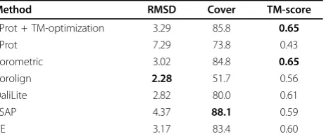
Quality of structural alignments

It would also be appropriate to investigate what is the quality of alignments and scores the measure produces. For this purpose, 10 difficult pairs of structures were intro-duced in [29]. It is obvious from Table 1 that SProt does not produce high alignment cover and TM-score. How-ever, to produce better alignment and TM-score, it is pos-sible to apply iterative improvement of TM-score. In this case, the superposition obtained by the original SProt is used to produce a new better alignment. A similar approach was utilized also by other methods, e.g., Voro-metric. For the purpose of the improvement, Needleman-Wunsch algorithm is used with the scoring function

S

d d L

ij

ij o T

dij do LT

= <

−∞ ⎧ ⎨ ⎪

⎩⎪

+

( )

1

2 3

( )

if

otherwise

(8)

where dij represents distance between i-th and j-th

amino acid according to the superposition, LT is the

length of the query protein, andd0(LT) is the scale func-tion used in TM-score. The 3d0(LT ) threshold is used to prevent aligning too distant amino acids. The result-ing alignment is then used in the TM-score algorithm to obtain new score and superposition. This procedure is repeated while the score is being improved.

As shown in Table 3, this approach (denoted SProt + TM-optimization) significantly improves the cover and score. On the other hand, extensive use of the iterative concept does not improve the results of the previous evaluations whereas it noticeably downgrades perfor-mance of the algorithm.

Efficiency

To evaluate the speedup possibilities based on indexing, we utilized the ProtDex2 dataset. This dataset is large enough to show advantages of indexing. On the other hand, it is still size that allows to perform the sequence

scan in a reasonable time. Hence results of sequence scan can be used for comparison.

The following settings were used. We selected 1651 protein structures as pivots, one from each family in the dataset. The value tolerance factor was set to 2.5% and the order tolerance factor was set to 128. The number of steps over which the pivots were protected against elimination was set to

1

64 _{of the total number of pivots.}

These settings provide sufficient robustness to prevent overvalued estimations for the used dataset.

A more important property is the impact of the employed modifiers that seamlessly balance between the retrieval accuracy and the speed. The SProt measure ranges from 0 to 1 while most of the distances (approxi-mately 95%) are higher than 0.7. Therefore, we decided on the basis of our experience to use a modifier that, simply said, smoothly expands the interval [0.7:1] at the expense of the interval [0:0.7] which is condensed. One of such modifiers is the RBQ(0.7,0.15)(w) modifier [26] parametrized by a weightw. This modifier is defined as the rational Bézier quadric curve, starting at point [0, 0] going toward point [0.7, 0.15] and arriving in point [1, 1]. The weightw determines the degree of deflection of the curve toward the point [0.7, 0.15] (i.e., the convexity

of the function). Thus, the weight w determines the

ratio of the expansion and condensation and thus it also impacts the indexability. The RBQ[0.7,0.15](w) modifier for various weightswis depicted in the Figure 3.

As shown in Figure 4, the computation time and the number of protein structure pairs being compared increases with the decreasing weight, and they also natu-rally increase with the increasing number of the requested nearest neighbors.

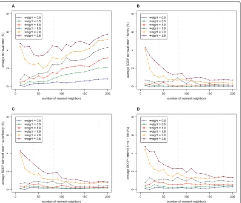
It is also important to describe the precision of such approximative searches. The precision of approximate search usingk-nearest neighbor query is measured as the retrieval errorbetween the query result returned by the SProt access method (R(q)) and the accurate query result obtained by sequential scan of the database (Rseq(q)):

Table 2 Average precision

Method Mean average precision

Average precision for standard recall levels

SProt 88.3 86.9

Vorometric n/a 82.91

CE 83.4 80.9

MAMMOTH 82.1 80.8

3D-BLAST 78.2 76.2

PSI-BLAST 69.8 61.8

The experiments was performed against the ProtDex2 dataset and all 108 queries were utilized. The mean average precision values of the compared methods are taken from [14], and the average precision for standard recall levels values of the compared methods are taken from [10].

1

based on returning top 100 hits

Table 3 Comparison of the alignment quality

Method RMSD Cover TM-score

SProt + TM-optimization 3.29 85.8 0.65

SProt 7.29 73.8 0.43

Vorometric 3.02 84.8 0.65

Vorolign 2.28 51.7 0.56

DaliLite 2.82 80.0 0.61

SSAP 4.37 88.1 0.59

CE 3.17 83.4 0.60

(10)

E R q R q R q

seq

seq = ( )− ( )

( ) . (9)

The retrieval error describes how many percent of structures included in the sequential scan result are missing in the result of the SProt access method.

As shown in Figure 5A, the retrieval error naturally increases with the increasing weight. Moreover, with the increasing number of the requested nearest neighbors, the error increases. An exception is the retrieval error for high weights and low numbers of the requested nearest neighbors, where it also increases. However, with the increasing number of the requested nearest neighbors, the retrieval error becomes less significant. The reason is that missing structures are often located in the back positions of the result. As shown in the information retrieval experiment, at the back positions there are located relatively few of the relevant structures (according to meaning of domain experts). So, we also introduce SCOP retrieval errors that takes into account the SCOP categories (family, superfamily or fold):

E

R q S q R q

R q S q R q S q

L

seq L

=

−

≠

( ( ) ( )) ( )

( ) ( ) ( ) ( )



 if 

oth

0

0 eerwise

⎧ ⎨ ⎪⎪

⎩ ⎪ ⎪

(10)

where R(q) is the result set obtained by the method for query q andRseq(q) is the sequential scan result set and SL(q) is a set of all structures having the same SCOP category at level L(at the family, superfamily or

fold level) as the query structure q. Thus, the SCOP

errors describe how many percent of relevant structures included in the sequential scan result are missing in the result of the SProt access method. As it can be seen in Figure 5, the SCOP errors still naturally increase with the increasing weight. Nevertheless, the errors do not negatively depend on the number of the requested near-est neighbors and they are very small. Again, the

original distance

modified distance

0.0 0.2 0.4 0.6 0.8 1.0

0.0

0.2

0.4

0.6

0.8

1.0

weight = 0.0 weight = 0.5 weight = 1.0 weight = 1.5 weight = 2.0 weight = 2.5

Figure 3RBQ modifiersRBQ(a,b)(w) modifier is defined as the

rational Bézier quadric curve starting at point [0, 0] going toward the control point [a,b] ([0.7, 0.15] in this case) and arriving to point [1, 1]. Weightwdetermines the degree of deflection of the curve toward the control point.

number of nearest neighbors

av

er

age n

umber of compared pairs (%)

0 50 100 150 200

0

102

03

04

05

0

A

av

er

age relativ

e computation time (%)

0 50 100 150 200

0

102

03

04

05

0

048

12

16

20

B

ave

ra

ge computation time

(min

)

(11)

exceptions are the errors for high weights and low num-bers of the requested nearest neighbors.

When searching in ProtDex2 dataset, we could con-clude that the weight value of the modifier set close to 1 results in reasonably fast retrieval and low retrieval errors. However, the optimal configuration of the SProt access methods parameters may vary, depending on the dataset used (especially on its size and indexability). However, it is important that the above factors (except from pivot selection) do not need to be know during the database indexing and can be set right at the query time. Thus, the user has the freedom to change the

settings if he is not satisfied with the obtained results, and run the query again using the same index.

Conclusions

In this paper, we proposed SProt –a novel algorithm

for measuring protein structure similarity that puts emphasis on high-quality modeling of local similarities of the amino acids. This is achieved by representing each amino acid by its spatial neighborhood containing close amino acids. The approach leads to good real-world results, especially for superfamily/fold classifica-tion accuracy and for precision at high recall levels

av

er

age retr

ie

val error (%)

0 50 100 150 200

02468

A

av

er

age SCOP retr

ie

val error

−

family (%)

0 50 100 150 200

02468

B

av

er

age SCOP retr

ie

val error

−

superf

amily (%)

0 50 100 150 200

02468

C

av

er

age SCOP retr

ie

val error

−

fold (%)

0 50 100 150 200

02468

D

(12)

where we outperform all the compared solutions. The focus on the quality of the modeling results in high computational demands of the method. We resolve this

handicap be introduction of SProt access method –a

modification of LAESA metric access method – that

highly decreases the runtime needed for scanning large datasets of protein structures. The speedup makes SProt competitive with the best contemporary solutions not only concerning the effectiveness but also the efficiency.

Authors contributions

JG designed and implemented both the measure and the access method. DH critically revised the both. JG per-formed all the measurements. JG and DH drafted the manuscript. TS critically revised the manuscript and gave final approval of the work to be published. All authors read and approved the final manuscript.

Abbreviations

ECDF: empirical cumulative distribution function; LAESA: linear

approximating and eliminating search algorithm; NP-hard: non-deterministic polynomial-time hard; PSI: percentage of structural identity; RBQ: rational Bézier quadratic; RMSD: root mean square deviation; SCOP: structural classification of proteins;

Acknowledgements

The work was supported by the Czech Science Foundation, project Nr. 201/ 09/0683 and by the Grant Agency of Charles University, project Nr. 430711 and by the grant SVV-2010-261312.

This article has been published as part ofProteome ScienceVolume 9 Supplement 1, 2011: Proceedings of the International Workshop on Computational Proteomics. The full contents of the supplement are available online at http://www.proteomesci.com/supplements/9/S1.

Competing interests

The authors declare that they have no competing interests.

Published: 14 October 2011

References

1. Lathrop RH:The protein threading problem with sequence amino acid interaction preferences is NP-complete.Protein Eng1994,7(9):1059-1068. 2. Kabsch W:A solution for the best rotation to relate two sets of vectors.

Acta Crystallogr A1976,32(5):922-923.

3. Holm L, Sander C:Protein structure comparison by alignment of distance matrices.J Mol Biol1993,233:123-138.

4. Holm L, Park J:DaliLite workbench for protein structure comparison.

Bioinformatics2000,16(6):566-567.

5. Aung Z, Tan KL:Rapid 3D protein structure database searching using information retrieval techniques.Bioinformatics2004,20(7):1045-1052. 6. Shindyalov IN, Bourne PE:Protein structure alignment by incremental combinatorial extension (CE) of the optimal path.Protein Eng1998,

11(9):739-747.

7. Taylor W, Flores T, Orengo C:Multiple protein structure alignment.Protein Sci1994,3(10):1858-1870.

8. Smith TF, Waterman MS:Identification of common molecular subsequences.J Mol Biol1981,147:195-197.

9. Ortiz AR, Strauss CE, Olmea O:MAMMOTH (matching molecular models obtained from theory): an automated method for model comparison.

Protein Sci2002,11(11):2606-2621.

10. Sacan A, Toroslu HI, Ferhatosmanoglu H:Integrated search and alignment of protein structures.Bioinformatics2008,24(24):2872-2879.

11. Birzele F, Gewehr JE, Csaba G, Zimmer R:Vorolign-fast structural alignment using Voronoi contacts.Bioinformatics2007,23(2):e205-e211.

12. Csaba G, Birzele F, Zimmer R:Protein structure alignment considering phenotypic plasticity.Bioinformatics2008,24(16):i98-i104.

13. Hoksza D, Galgonek J:Density-Based Classification of Protein Structures Using Iterative TM-score.InBIBMW: 2009 IEEE International Conference on Bioinformatics and Biomedicine WorkshopChen J, Chen X, Ely J, Hakkanitr D, He J and Hsu HH 2009, 85-90[http://dx.doi.org/10.1109/

BIBMW.2009.5332142].

14. Tung CHH, Huang JWW, Yang JMM:Kappa-alpha plot derived structural alphabet and BLOSUM-like substitution matrix for rapid search of protein structure database.Genome Biol2007,8(3):R31+.

15. Altschul SF, Gish W, Miller W, Myers EW, Lipman DJ:Basic local alignment search tool.J Mol Biol1990,215(3):403-410.

16. Altschul SF, Madden TL, Schäffer AA, Zhang J, Zhang Z, Miller W, Lipman DJ:Gapped BLAST and PSI-BLAST: a new generation of protein database search programs.Nucleic Acids Res1997,25(17):3389-3402. 17. Needleman SB, Wunsch CD:A general method applicable to the search

for similarities in the amino acid sequence of two proteins.J Mol Biol

1970,48(3):443-453.

18. Zhang Y, Skolnick J:Scoring function for automated assessment of protein structure template quality.Proteins2004,57(4):702-710. 19. Siew N, Elofsson A, Rychlewski L, Fischer D:MaxSub: an automated

measure for the assessment of protein structure prediction quality.

Bioinformatics2000,16(9):776-785.

20. Cristobal S, Zemla A, Fischer D, Rychlewski L, Elofsson A:A study of quality measures for protein threading models.BMC Bioinformatics2001,2:5+. 21. Chandonia J, Hon G, Walker N, Conte L, Koehl P, Levitt M, Brenner S:The

ASTRAL Compendium in 2004.Nucleic Acids Res2004,32(Database issue): D189-D192.

22. Chávez E, Navarro G, Baeza-Yates RA, Marroquín JL:Searching in metric spaces.ACM Comput. Surv2001,33(3):273-321.

23. Micó ML, Oncina J, Vidal E:A new version of the nearest-neighbour approximating and eliminating search algorithm (AESA) with linear preprocessing time and memory requirements.Pattern Recognition Letters

1994,15:9-17.

24. Moreno-Seco F, Micó L, Oncina J:Extending LAESA Fast Nearest Neighbour Algorithm to Find the k Nearest Neighbours.Proceedings of the Joint IAPR International Workshop on Structural, Syntactic, and Statistical Pattern Recognition2002, 718-724[http://dl.acm.org/citation.cfm?id=671268]. 25. Skopal T, Loko_čJ, Bustos B:D-cache: Universal Distance Cache for Metric

Access Methods.IEEE Transactions on Knowledge and Data Engineering

2011,99: [http://doi.ieeecomputersociety.org/10.1109/TKDE.2011.19], (PrePrints).

26. Skopal T:Unified framework for fast exact and approximate search in dissimilarity spaces.ACM Trans. Database Syst2007,32(4):19-28[http://dl. acm.org/citation.cfm?id=1292619].

27. Murzin AG, Brenner SE, Hubbard T, Chothia C:SCOP: a structural classification of proteins database for the investigation of sequences and structures.J Mol Biol1995,247(4):536-540.

28. Baeza-Yates RA, Ribeiro-Neto BA:Modern Information Retrieval.ACM Press / Addison-Wesley; 1999.

29. Fischer D, Elofsson A, Rice D, Eisenberg D:Assessing the performance of fold recognition methods by means of a comprehensive benchmark.Pac Symp Biocomput1996, 300-18.

30. Humphrey W, Dalke A, Schulten K:VMD: visual molecular dynamics.J Mol Graph1996,14:33-38.

doi:10.1186/1477-5956-9-S1-S20