VALUING CREDIT DEFAULT SWAPS I: NO COUNTERPARTY DEFAULT RISK
John Hull and Alan White
Joseph L. Rotman School of Management University of Toronto
105 St George Street Toronto, Ontario M5S 3E6
Canada
Tel: (416) 978 8615 (Hull) Tel: (416) 978 3689 (White)
VALUING CREDIT DEFAULT SWAPS I: NO COUNTERPARTY DEFAULT RISK
Abstract
Credit default swaps have become increasingly popular in recent years. Their purpose is to allow credit risks to be traded and managed in much the same way as market risks. In 1998, trading in credit default swaps was facilitated by standard documentation produced by the International Swaps and Derivatives Association.
A credit default swap (CDS) is a contract that provides insurance against the risk of a default by particular company. The company is known as the reference entity and a default by the company is known as a credit event. The buyer of the insurance obtains the right to sell a particular bond issued by the company for its par value when a credit event occurs. The bond is known as the reference obligation and the total par value of the bond that can be sold is known as the swap’s notional principal.
The buyer of the CDS makes periodic payments to the seller until the end of the life of the CDS or until a credit event occurs. A credit event usually requires a final accrual payment by the buyer. The swap is then settled by either physical delivery or in cash. If the terms of the swap require physical delivery, the swap buyer delivers the bonds to the seller in exchange for their par value. When there is cash settlement, the calculation agent polls dealers to determine the mid-market price, Q, of the reference obligation some specified number of days after the credit event. The cash settlement is then (100−Q)% of the notional principal.
million. If the contract requires cash settlement, the calculation agent would poll dealers to determine the mid-market value of the reference obligation a predesignated number of days after the credit event. If the value of the reference obligation proved to be $35 per $100 of par value, the cash payoff would be $65 million. In the case of either physical or cash settlement, the buyer would be required to pay to the seller the amount of the annual payment accrued between March 1, 2003 and September 1, 2003 (approximately $450,000), but no further payments would be required.
There are a number of variations on the standard credit default swap. In a binary credit default swap, the payoff in the event of a default is a specific dollar amount. In a basket credit default swap, a group of reference entities are specified and there is a payoff when the first of these reference entities defaults. In acontingent credit default swap, the payoff requires both a credit event and an additional trigger. The additional trigger might be a credit event with respect to another reference entity or a specified movement in some market variable. In adynamic credit default swap, the notional amount determining the payoff is linked to the mark-to-market value of a portfolio of swaps.
In this paper we explain how a plain vanilla and binary credit default swap can be val-ued assuming no counterparty default risk. Like most other approaches, ours assumes that default probabilities, interest rates, and recovery rates are independent. Unfortunately, it does not seem to be possible to relax these assumptions without a considerably more complex model. However, we are able to reach some general conclusions about the impact of the assumptions on CDS valuations.
1. Estimation of Default Probabilities
The valuation of a credit default swap requires estimates of the risk-neutral probability that the reference entity will default at different future times. The prices of bonds issued by the reference entity provide the main source of data for the estimation. If we assume that the only reason a corporate bond sells for less than a similar Treasury bond is the possibility of default, it follows that:
Value of Treasury Bond−Value of Corporate Bond = Present Value of Cost of Defaults
By using this relationship to calculate the present value of the cost of defaults on a range of different bonds issued by the reference entity, and making an assumption about recovery rates, we can estimate the probability of the corporation defaulting at different future times.1 If the reference entity has issued relatively few actively traded bonds, we can use bonds issued by another corporation that is considered to have the same risk of default as the reference entity. This is likely to be a corporation whose bonds have the same credit rating as those of the reference entity—and ideally a corporation in the same industry as the reference entity.
We start with a simple example. Suppose that a five-year zero-coupon Treasury bond with a face value of 100 yields 5% and a similar five-year zero-coupon bond issued by a corporation yields 5.5%. (Both rates are expressed with continuous compounding.) The value of the Treasury bond is 100e−0.05×5 or 77.8801 and the value of the corporate bond is 100e−0.055×5 = 75.9572. The present value of the cost of defaults is, therefore
77.8801−75.9572 = 1.9229
default, the impact of a default is to create a loss of 100 at the end of the five years. The expected loss from defaults in a risk-neutral world is, therefore, 100pand the present value of the expected loss is
100pe−0.05×5
It follows that:
100pe−0.05×5 = 1.9229
so that p= 0.0247 or 2.47%.
There are two reasons why the calculations for extracting default probabilities from bond prices are, in practice, usually more complicated than this. First, the recovery rate is usually non-zero. Second, most corporate bonds are not zero-coupon bonds.
When the recovery rate is non-zero, it is necessary to make an assumption about the claim made by bondholders in the event of default. Jarrow and Turnbull (1995) and Hull and White (1995) assume that the claim equals the no-default of the bond. Duffie and Singleton (1997) assume that the claim is equal to the value of the bond immediately prior to default. As pointed out by J.P. Morgan (1999) and Jarrow and Turnbull (2000), these assumptions do not correspond to the way bankruptcy laws work in most countries. The best assumption is that the claim made in the event of a default equals the face value of the bond plus accrued interest.
As mentioned earlier, the payoff from a CDS in the event of a default at time t is usually the face value of the reference obligation minus its market value just after time t. Using the best claim amount assumption just mentioned, the market value of the reference obligation just after default is the recovery rate times the sum of its face value and accrued interest. This means that the payoff from a typical CDS is
L−RL[1 +A(t)] =L[1−R−A(t)] (1)
A General Analysis Assuming Defaults at Discrete Times
We now present a general analysis that can be used in conjunction with alternative assumptions about the claim amount. We assume that we have chosen a set of N bonds that are either issued by the reference entity or issued by another corporation that is considered to have the same risk of default as the reference entity.2 We assume that defaults can happen on any of the bond maturity dates. Later we generalize the analysis to allow defaults to occur on any date. Suppose that the maturity of the ith bond is ti with t1 < t2 < t3... < tN. Define:
Bj: Price of the jth bond today
Gj: Price of the jth bond today if there were no probability of default (that is, the price of a Treasury bond promising the same cash flows as the jth bond).
Fj(t): Forward price of thejth bond for a forward contract maturing at time tassuming the bond is default-free (t < tj)
v(t): Present value of $1 received at time t with certainty
Cj(t): Claim made by holders of thejth bond if there is a default at timet (t < tj) Rj(t): Recovery rate for holders of the jth bond in the event of a default at time t
(t < tj)
αij: Present value of the loss, relative to the value the bond would have if there were no possibility of default, from a default on the jth bond at time ti
pi: The risk-neutral probability of default at time ti
For ease of exposition, we first assume that interest rates are deterministic and that both recovery rates and claim amounts are known with certainty. We then explain how these assumptions can be relaxed.
Because interest rates are deterministic, the price at time t of the no-default value of
the jth bond is Fj(t). If there is a default at time t, the bondholder makes a recovery at rate Rj(t) on a claim of Cj(t). It follows that
αij =v(ti)[Fj(ti)−Rj(ti)Cj(ti)] (2)
There is a probability,pi of the lossαij being incurred. The total present value of the losses on the jth bond is, therefore, given by:
Gj−Bj = j
X
i=1
piαij (3)
This equation allows the p’s to be determined inductively:
pj =
Gj−Bj−Pj−1
i=1 piαij
αjj (4)
Recovery Rate Assumption
These results have been produced on the assumption that interest rates are constant, recovery rates are known, and claim amounts are known. In what follows we will consider two assumptions about the claim amount. The first is that it equals the no-default value of the bond at the time of the default; the second is that it equals the face value plus accrued interest at the time of the default. It can be shown that, for either of these two assumptions, if a) default events, b) Treasury interest rates, and c) recovery rates are mutually independent, equations (2) and (3) are still true for stochastic interest rates, uncertain recovery rates, and uncertain default probabilities providing the recovery rate is set equal to its expected value in a risk-neutral world.
be expected, the mean recovery rate is heavily dependent on the seniority of the bond. As mentioned earlier, the N bonds used in the analysis are issued either by the ref-erence entity or by another company that is considered to have the same risk of default as the reference entity. This means that the pi should be the same for all bonds. The recovery rates can in theory vary according to the bond and the default time. We will assume, for ease of exposition, that all the bonds have the same seniority in the event of default by the reference obligation and that the expected recovery rate is independent of time. The expected value of Rj(t) is then independent of both j and t. We will denote this expected value by ˆR.
Extension to Situation Where Defaults can Happen at any Time
The analysis used to derive equation (4) assumes that default can take place only on bond maturity dates. We now extend it to allow defaults at any time. Define q(t)∆t as the probability of default between times t and t+ ∆t as seen at time zero. The variable q(t) is not the same as the hazard (default intensity) rate. The hazard rate,h(t), is defined so that h(t)∆t is the probability of default between times t and t+ ∆t as seen at time t assuming no default between time zero and time t. The variablesq(t) and h(t) are related by
q(t) =h(t)e−
Rt 0 h(τ)dτ
Many credit risk models such as Duffie and Singleton (1997), Jarrow and Turnbull (1995), and Lando (1998) are formulated in terms of h(t). However, we find it convenient to express our results in terms of q(t) rather than h(t). We will refer to q(t) as the default probability density.
We assume that q(t) is constant and equal to qi for ti−1 < t < ti.4. Setting
βij =
Z ti
ti−1
v(t)[Fj(t)−RCj(t)]dtˆ (5)
a similar analysis to that used in deriving equation (4) gives:
qj = Gj −Bj −
Pj−1
i=1 qiβij βjj
(6)
The parameters βij can be estimated using standard procedures, such as Simpson’s rule, for evaluating a definite integral.
Claim Amounts and Value Additivity
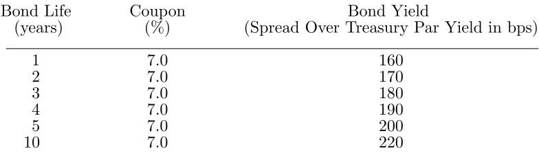
We now present a numerical example and investigate the impact of different assump-tions about the claim amount. As mentioned earlier, Jarrow and Turnbull (1995) and Hull and White (1995) assume that, in the event of a default, the bondholder claims the no-default value of the bond. This is an attractive assumption. It implies that Cj(t) =Fj(t). The parameter, βij, is then proportional to 1−Rˆ so that equation (6) can be used to estimate qi(1−R) directly from observable market variables. Furthermore, an analysis ofˆ equation (6) shows that, in this case, the value of the coupon-bearing bondBj is the sum of the values of the underlying zero-coupon bonds. This property is referred to as value additivity. It implies that it is theoretically correct to calculate zero curves for different rating categories (AAA, AA, A, BBB, etc) from actively traded bonds and use them for pricing less actively traded bonds.
As mentioned earlier, the best assumption is that Cj(t) equals the face value of bond j plus accrued interest at time t. As pointed out by Jarrow and Turnbull (2000), value additivity does not apply when this assumption is made (except in the special case where the recovery rate is zero). This means that there is no zero-coupon yield curve that can be used to price corporate bonds exactly for a given set of assumptions about default probabilities and expected recovery rates.
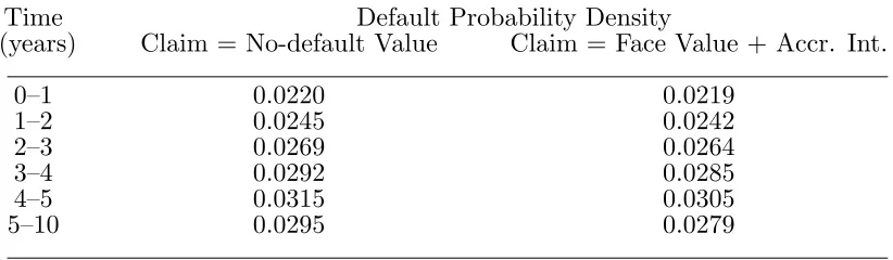
compounded), and the expected recovery rate is assumed to be 30%. Table 3 calculates the default probability densities for the two alternative assumptions about the claim amount. It can be seen that the two assumptions give similar results. This is usually the case. For the default probability densities to be markedly different, it would be necessary for the coupons on the bonds to be either very much greater or very much less than the risk-free rate.5
Expected Recovery Rates and Bond Yields
Default probability densities must be greater than zero. From equation (6) this means that
Bj ≤Gj − j−1
X
i=1
qiβij (7)
It is also true that the cumulative probability of default must be less than 1. This means that
j
X
i=1
qi(ti−ti−1)≤1
or
qj(tj−tj−1)≤1− j−1
X
i=1
qi(ti−ti−1)
so that from equation (6)
Bj ≥Gj −
j−1
X
i=1
qiβij− βjj
tj −tj−1
"
1−
j−1
X
i=1
qi(ti−ti−1)
#
(8)
Equations (7) and (8) impose both an upper and lower bound on the yield on the bond maturing at time tj once expected recovery rates and the yields on bonds maturing at earlier times have been specified. In the example in Table 2, when the expected recovery rate is 30%, a 20-year bond with a coupon of 7% must have a yield between 6.50% and 9.57% when the claim amount equals the face value plus accrued interest.
2. The Valuation
We now move on to consider the valuation of a plain vanilla credit default swap with a $1 notional principal. We assume that default events, Treasury interest rates, and recovery rates are mutually independent. We also assume that the claim in the event of default is the face value plus accrued interest. Define
T: Life of credit default swap
q(t): Risk-neutral default probability density at time t ˆ
R: Expected recovery rate on the reference obligation in a risk-neutral world. As indicated in the previous section, this is assumed to be independent of the time of the default and the same as the recovery rate on the bonds used to calculate q(t).
u(t): Present value of payments at the rate of $1 per year on payment dates between time zero and timet
e(t): Present value of an accrual payment at time t equal to t−t∗ wheret∗ is the payment date immediately preceding time t.
v(t): Present value of $1 received at time t
w: Total payments per year made by credit default swap buyer
s: Value of w that causes the credit default swap to have a value of zero π: The risk-neutral probability of no credit event during the life of the swap
A(t): Accrued interest on the reference obligation at time t as a percent of face value The value of π is one minus the probability that a credit event will occur by time T. It can be calculated from q(t):
π = 1− Z T
0
q(t)dt
value of the payments is, therefore:
w
Z T
0
q(t)[u(t) +e(t)]dt+wπu(T)
Given our assumption about the claim amount, equation (1) shows that the risk-neutral expected payoff from the CDS is
1−[1 +A(t)] ˆR= 1−Rˆ−A(t) ˆR
The present value of the expected payoff from the CDS is
Z T
0
[1−Rˆ−A(t) ˆR]q(t)v(t)dt
and the value of the credit default swap to the buyer is the present value of the expected payoff minus the present value of the payments made by the buyer or
Z T
0
[1−Rˆ−A(t) ˆR]q(t)v(t)dt−w
Z T
0
q(t)[u(t) +e(t)]dt−πwu(T)
The CDS spread, s, is the value ofw that makes this expression zero:
s=
RT
0 [1−Rˆ−A(t) ˆR]q(t)v(t)dt
RT
0 q(t)[u(t) +e(t)]dt+πu(T)
(9)
The variable s is referred to as the credit default swap spreador CDS spread. It is the total of the payments per year, as a percent of the notional principal, for a newly issued credit default swap. Consider the data in Table 2 and suppose that the reference obligation is a five-year bond paying a semiannual coupon of 10% per annum with ˆR= 0.3. Equation (9) gives the value ofs for a five-year credit default swap with semiannual payments to be 1.944%. This is an annualized spread because of the way w is defined. Payments equal to 0.972% of the CDS notional principal would be required every six months.
Approximate No-Arbitrage Arguments
the reference entity and the credit default swap, the investor has eliminated most of the risks associated with default on the bond. If y is the yield to maturity on the bond, the investor’s net annual return is (at least, approximately) y−s. In the absence of arbitrage opportunities this should be (again, approximately) the T-year Treasury par yield, which we will denote by x. If y− s is significantly higher than x, an arbitrageur will find it profitable to buy a T-year par yield bond issued by the reference entity, buy the credit default swap, and short a T-year par yield Treasury bond. If y−s is significantly less thanx, an arbitrageur will find it profitable to short aT-year par yield bond issued by the reference entity, sell the credit default swap, and buy a T-year Treasury par yield bond.
The argument just given suggests thatsshould equal y−x. However, a close analysis of it shows that the arbitrage is less than perfect. Define:
s∗ : y−x
L: CDS notional principal
A∗(t): The accrued interest as a percent of the face value at time t on a T-year par yield bond that is issued at time zero by the reference entity with the same payment dates as the swap. We will refer to this bond as the underlying par yield corporate bond.
R: Realized recovery rate when a default happens
from the CDS is
L[1 +A∗(t)](1−R)−L(y−x)(t−t∗)
where as before t∗ is the payment date immediately prior to time t. Because A∗(t) = y(t−t∗), this reduces to
L[1 +x(t−t∗)]−LR[1 +A∗(t)]
The corporate bond holding is worth LR[1 +A∗(t)] so that the net value of the holding is L[1 +x(t−t∗)]. This is exactly what is required to buy a par yield Treasury bond with a face value of L at time t. It follows that in all circumstances, the investor’s portfolio exactly replicates the cash flows from the par yield Treasury bond showing that s∗ must be the correct CDS spread. A spread greater than or less than s∗ would give rise to an arbitrage opportunity.
We will refer to a CDS that provides a payoff of [1 +A∗(t)](1−R) as an idealized credit default swap. Our analysis shows that the spread on such a CDS is exactly s∗. In practice, the payoff from a credit default swap is usually 1−R−A(t)R rather than [1 +A∗(t)](1−R). This leads tos∗ overestimating the true spread, s.
Continuing for a moment with the assumption that the Treasury curve is flat and interest rates are constant, we can correct for the difference between the payoff on the idealized CDS and the actual CDS. An analysis similar to that leading up to equation (9) shows that the spread for an idealized credit default swap is given by
s∗ = (1− ˆ
R)R0T[1 +A∗(t)]q(t)v(t)dt
RT
0 q(t)[u(t) +e(t)]dt+πu(T) An approximation to this is
s∗ = (1− ˆ
R)(1 +a∗)R0T q(t)v(t)dt
RT
0 q(t)[u(t) +e(t)]dt+πu(T)
(10)
where a∗ is the average value of A∗(t) for 0 ≤ t ≤ T. Similarly, from equation (9), an approximation to the actual CDS spread is
s= (1− ˆ
R−aR)ˆ R0T q(t)v(t)dt
RT
0 q(t)[u(t) +e(t)]dt+πu(T)
where a is the average value of A(t) for 0 ≤t ≤T. From equations (9) and (10)
s= s
∗(1−Rˆ−aR)ˆ
(1−R)(1 +ˆ a∗) (12)
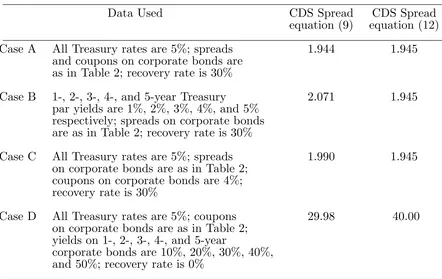
As an illustration of equation (12), consider the data in Table 2 and assume, as before, that the coupon on the reference obligation is 10%. (We will refer to this as Case A; see Table 4.) The five-year par yield for bonds issued by the reference entity is 7%. The five-year Treasury par yield is 5%. It follows that, for a five-year credit default swap with semiannual payments,s∗ is 2.00%. The coupon paid every six months on a par yield bond issued by the reference entity is 3.5 per 100 of principal so thata∗ = 0.0175. Alsoa= 0.025 and ˆR = 0.3 so that equation (12) gives s = 1.945%. This is very close to the 1.944% estimate reported earlier from using equation (9).
Equation (12) assumes a flat Treasury yield curve and constant interest rates. Stochas-tic interest rates make the no-arbitrage argument for the idealized CDS less than perfect, but do not affect valuations given our assumption that interest rates, default probabilities, and recovery rates are independent. However, the no-arbitrage argument for the idealized CDS swap requires a flat yield curve so that a par yield Treasury bond is always worth its face value plus accrued interest at the time of a default. An upward sloping yield curve will lead to the par yield Treasury bond being worth less than the face value plus accrued interest on average. As a result s∗ underestimates the spread for the idealized CDS. Simi-larly a downward sloping yield curve leads tos∗ overestimating the spread on the idealized CDS.
floater for the life of the credit default swap. If the payoff from the credit default swap is [1 +A∗(t)](1−R) where A∗(t) is here defined as the accrual on the par floater issued by the reference entity, the arbitrage arguments are watertight and the CDS spread should exactly equal the spread of the reference entity floater over the Treasury floater.
In practice we rarely get the opportunity to observe the spreads on corporate par yield floaters. Credit default swaps must be evaluated from the yields on fixed rate bonds issued by the reference entity. The difference between the spread on par yield floaters and par yield fixed rate instruments is very small for flat term structures, but noticeable for non-flat term structures. As an extreme test of the effect of a non-flat term structure we changed the flat Treasury curve in Case A to a Treasury curve where the 1-, 2-, 3-, 4-, and 5-year par yields were 1%, 2%, 3%, 4%, and 5%, respectively. (We will refer to this as Case B; see Table 4.) Everything else, including the spreads between par yields on Treasuries and yields on bonds issued by the reference entity was maintained as in Case A. As a result, the five-year par yield for bonds issued by the reference was still 7% and s∗ was still 2.00%. However, the value of s given by equation (9) increased from 1.944% to 2.071%.
We also rarely get the chance to observe corporate bonds that are selling for exactly their par value. Assuming that the yield on a non-par-yield bond is the same as the yield on a par yield bond introduces some error. We tested this by changing the coupons on all bonds used to calculate default probabilities in Case A from 7% to 4% while keeping everything else (including the yield on the bonds) the same as in Case A. (We will refer to this as Case C; see Table 4.) The value of s increased from 1.944 to 1.990. This change results entirely from the correct five year par yield being 7.048% rather than 7%.6 For less creditworthy reference entities, the error from basing calculations on non-par-yield bonds
can be much greater. Suppose Case A is changed so that the recovery rate is zero and the 1-, 2-, 3-, 4-, and 5-year yields on bonds issued by the reference entity are 10%, 20% 30%, 40% and 50%, respectively. (We will refer to this as Case D; see Table 4.) Assuming that the par yield is 50% and using equation (12) leads to an estimate of 40% for the value ofs (s∗ = 45, a∗ = 0.125,a= 0.025, and ˆR= 0). The correct value ofs given by equation (9) is 29.98%. This difference largely results from the correct par yield being about 38% rather than 50%. Impact of Expected Recovery Rate on Pricing
The one parameter necessary for valuing a credit default swap that cannot be observed directly in the market is the expected recovery rate. We assume that the same recovery rate is used for estimating the default probability densities and for calculating the payoff. As it happens there is an offset. As the expected recovery rate increases, estimates of the probability of default increase and payoffs decrease. The overall impact of the recovery rate assumption on the value of a credit default swap is generally fairly small when the expected recovery rate is in the 0% to 50% range.
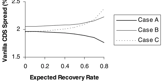
This is illustrated in Figure 1, which shows the dependence of the five-year CDS spread on the expected recovery rate in Cases A, B, and C considered above.7 In Case A the yield curve is flat and the par yield spread is 2%. The spread for an idealized CDS,s∗, is always exactly 2%. The actual CDS spread is less than 2% and is a decreasing function of the expected recovery rate. When we move from Case A to the upward sloping yield curve in Case B, the CDS spread increases. The higher the expected recovery rate, the greater the impact of an upward sloping yield curve on the CDS spread. In Case C the coupon on the five year bond is less than the five-year par yield. This leads to the par yield being an increasing function of the expected recovery rate. As a result the CDS spread is also an increasing function of the expected recovery rate.
Binary Credit Default Swaps
A binary credit default swap is structured similarly to a regular credit default swap except that the payoff is a fixed dollar amount. A similar analysis to that given earlier shows that the value a binary CDS spread that provides a payoff of $1 in the event of a default is
RT
0 q(t)v(t)dt
RT
0 q(t)[u(t) +e(t)]dt+πu(T)
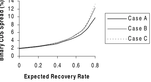
This is quite heavily dependent on the expected recovery rate, as illustrated by Figure 2. The Independence Assumptions
The valuation approaches we have presented are based on the assumption that inter-est rates, default probabilities, and recovery rates are independent. These assumptions are unlikely to be perfectly true in practice. For example, it can be argued that high interest rates cause companies to experience financial difficulties and, as a result, default probabil-ities increase. Such a positive relation between interest rates and default probabilprobabil-ities has two effects. First, high default probabilities tend to be associated with high discount rates for the payoffs. This reduces the CDS spread. Second high default probabilities tend to be associated with relatively low market values for bonds issued by the reference entity. This increases the CDS spread (because it increases the value of the buyer’s right to sell the reference bond for its face value). It is reassuring that these effects act in opposite directions so there is a partial offset. Note that the relevant correlation for the first effect is between default rates at time t and the average short term interest rates between time zero and time t; the relevant correlation for the second effect is between interest rates at time t and medium to long rates at time t. As far as the second effect is concerned, the correlation is less than might be supposed because there are often significant time lags between the occurrence of high interest rates and the resultant defaults.8
3. Application to Real Data
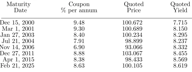
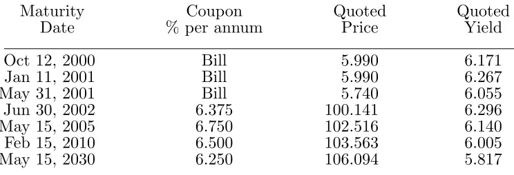
Up to now our illustrations of the methodology have been somewhat idealized. We now apply the approach to a real-world data. We consider the valuation of credit default swaps on Ashland Inc. at the close of trading on July 13, 2000. Ashland is a Fortune 500 company based in Kentucky with interests in chemicals, oil, car products, petroleum refining and retailing, and coal. The company had about 80 unsecured bonds outstanding on July 13, 2000. We did not have data on the volume of trading for the bonds and chose to base our analysis on quotes for a sample of eight of the bonds that had a wide range of maturities and relatively high issue sizes. Quotes for these bonds at the close of trading on July 13, 2000 are shown in Table 5. All bonds in our sample are all rated BBB by S&P and Baa2 by Moody’s. They contain no embedded options apart from a poison put. Quotes for the benchmark Treasury bonds and Treasury bills at the close of trading on July 13, 2000 are shown in Table 6.
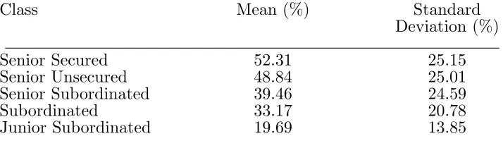
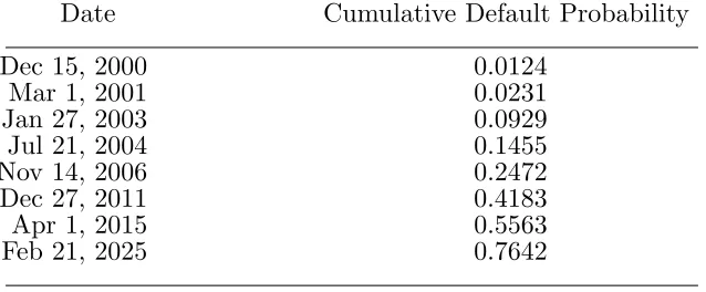
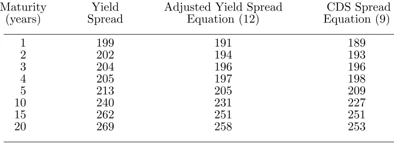
We used a bootstrap procedure to calculate a Treasury zero curve from the data in Table 6. We then estimated the default probabilities shown in Table 7 using the approach in Section 1. This in turn enabled us to use the approach in Section 2 to calculate CDS spreads for instruments with semiannual payments and a number of different maturities. The reference obligation was assumed to have a coupon of 8% per annum paid semiannually. From Table 1 we estimated the expected recovery rate to be 48.84%. Table 8 shows the CDS spreads together with
(a) The spread between Treasury yields and Ashland yields; and
(b) The spread between Treasury yields and Ashland yields after the adjustment in equa-tion (12) is applied
To make the adjustment in (b), A∗(t) was estimated by bootstrapping a zero curve for Ashland and using it to calculate par yields. This involved using the bootstrap method to calculate a zero curve for Ashland and using this to calculate the par yields. There is a very small approximation here because, as mentioned in Section 1, value additivity does not apply to corporate bonds.
4. Conclusions
The valuation of a credit default swap is a two step procedure. First bonds issued by the reference entity (or a company with the same risk of default as the reference entity) must be used to estimate the risk-neutral probability of the reference entity defaulting at different future times. The present value of the expected payments made by the buyer of the swap and the present value of the expected payoff must then be calculated.
The valuation requires estimates of the amount claimed by bondholders in the event of a default and the expected recovery rate. The most realistic assumption about the amount claimed in the event of a default is that it equals the face value of the bond plus accrued interest. The expected recovery rate must be estimated from empirical data. The valuation of a vanilla CDS is relatively insensitive to the expected recovery rate, but this is not so for a binary CDS.
REFERENCES
Duffie, D. “Credit Swap Valuation,”Financial Analysts Journal, (January/February 1999), 73–87.
Duffie, D. and K. J. Singleton, “An Econometric Model of the Term Structure of Interest-Rate Swap Yields,” Journal of Finance52, 1 (September 1997), 1287–1321. Hull, J. C. and A. White, “The Impact of Default Risk on Options and Other Deriva-tive Securities,” Journal of Banking and Finance, 19,2 (1995), 299–322.
Hull, J. C. and A. White, “Valuing Credit Default Swaps II: Modeling Default Cor-relations,” Working Paper in progress, University of Toronto, 2000.
Jarrow, R. A. and S. Turnbull, “Pricing Options on Derivative Securities Subject to Credit Risk,” Journal of Finance, 50, 1, (1995), 53–85.
Jarrow, R. A. and S. Turnbull, “The Intersection of Market and Credit Risk,”Journal of Banking and Finance, 24 (2000), 271–299.
J.P. Morgan, The J.P. Morgan Guide to Credit Derivatives, Risk Publications, 1999.
Lando, D., “On Cox Processes and Credit Risky Securities”, Review of Derivatives Research, 2 (1998), 99–120.
Table 1
Recovery Rates on Corporate Bonds from Moody’s Investor’s Service (2000)
Class Mean (%) Standard
Deviation (%)
Senior Secured 52.31 25.15
Senior Unsecured 48.84 25.01
Senior Subordinated 39.46 24.59
Subordinated 33.17 20.78
Table 2
Hypothetical Example of Bonds Issued by Reference Entity∗
Bond Life Coupon Bond Yield
(years) (%) (Spread Over Treasury Par Yield in bps)
1 7.0 160
2 7.0 170
3 7.0 180
4 7.0 190
5 7.0 200
10 7.0 220
∗Bond coupon is paid semiannually and bond yield is expressed with semiannual
Table 3
Implied Probabilities of Default for Data in Table 2 Time Default Probability Density
(years) Claim = No-default Value Claim = Face Value + Accr. Int.
0–1 0.0220 0.0219
1–2 0.0245 0.0242
2–3 0.0269 0.0264
3–4 0.0292 0.0285
4–5 0.0315 0.0305
Table 4 Cases Considered∗
Data Used CDS Spread CDS Spread
equation (9) equation (12) Case A All Treasury rates are 5%; spreads 1.944 1.945
and coupons on corporate bonds are as in Table 2; recovery rate is 30%
Case B 1-, 2-, 3-, 4-, and 5-year Treasury 2.071 1.945 par yields are 1%, 2%, 3%, 4%, and 5%
respectively; spreads on corporate bonds are as in Table 2; recovery rate is 30%
Case C All Treasury rates are 5%; spreads 1.990 1.945 on corporate bonds are as in Table 2;
coupons on corporate bonds are 4%; recovery rate is 30%
Case D All Treasury rates are 5%; coupons 29.98 40.00 on corporate bonds are as in Table 2;
yields on 1-, 2-, 3-, 4-, and 5-year
corporate bonds are 10%, 20%, 30%, 40%, and 50%; recovery rate is 0%
∗ Coupons are paid semiannually and all rates and yields are expressed with semiannual
Table 5
Quotes for Unsecured Bonds Issued By Ashland Inc. at Close of Trading on July 13, 2000
Maturity Coupon Quoted Quoted
Date % per annum Price Yield
Dec 15, 2000 9.48 100.672 7.715
Mar 1, 2001 9.30 100.689 8.150
Jan 27, 2003 8.40 100.234 8.295
Jul 21, 2004 7.91 98.899 8.237
Nov 14, 2006 6.90 93.066 8.332
Dec 27, 2011 8.88 103.067 8.455
Apr 1, 2015 8.38 98.433 8.569
Feb 21, 2025 8.63 100.105 8.619
Table 6
Quotes for Benchmark Government Bills and Bonds at Close of Trading on July 13, 2000
Maturity Coupon Quoted Quoted
Date % per annum Price Yield
Oct 12, 2000 Bill 5.990 6.171
Jan 11, 2001 Bill 5.990 6.267
May 31, 2001 Bill 5.740 6.055
Jun 30, 2002 6.375 100.141 6.296
May 15, 2005 6.750 102.516 6.140
Feb 15, 2010 6.500 103.563 6.005
May 15, 2030 6.250 106.094 5.817
Table 7
Cumulative Risk-Neutral Default Probabilities for Ashland Inc. Date Cumulative Default Probability
Dec 15, 2000 0.0124
Mar 1, 2001 0.0231
Jan 27, 2003 0.0929
Jul 21, 2004 0.1455
Nov 14, 2006 0.2472
Dec 27, 2011 0.4183
Apr 1, 2015 0.5563
Table 8
CDS Spreads for Ashland and Estimates Provided by the Yield Spread Before and After Applying the Adjustment in Equation (12) Maturity Yield Adjusted Yield Spread CDS Spread
(years) Spread Equation (12) Equation (9)
1 199 191 189
2 202 194 193
3 204 196 196
4 205 197 198
5 213 205 209
10 240 231 227
15 262 251 251
1.5 2 2.5
0 0.2 0.4 0.6 0.8
Expected Recovery Rate
V
a
n
il
la
C
D
S
S
p
re
a
d
(
%
)
Case A
Case B
[image:34.612.142.420.244.388.2]Case C
Figure 1
Dependence of Five-Year Credit Default Swap Spread on the Expected Recovery Rate When Reference Liability is a Five-Year 10% Coupon Bond
Case A: Data as in Table 2
Case B: Data as in Table 2 except that one-, two-, three-, four-, and five-year Treasury par yields are 1%, 2%, 3%, 4%, and 5%, respectively
0 2 4 6 8 1 0 1 2 1 4
0 0 .2 0 .4 0 .6 0 .8
Ex pe c te d Re c ove ry Ra te
B in a ry C D S S p re a d ( % )
C a s e A
C a s e B
[image:35.612.151.413.240.382.2]C a s e C
Figure 2
Dependence of Five-Year Binary Credit Default Swap Spread on the Expected Recovery Rate
Case A: Data as in Table 2
Case B: Data as in Table 2 except that one-, two-, three-, four-, and five-year Treasury par yields are 1%, 2%, 3%, 4%, 5%, respectively