Continuous wavelet transform and Euler deconvolution method and their application to magnetic field data of Jharia coalfield, India

www.geosci-instrum-method-data-syst.net/6/53/2017/ doi:10.5194/gi-6-53-2017

© Author(s) 2017. CC Attribution 3.0 License.

Continuous wavelet transform and Euler deconvolution method and

their application to magnetic field data of Jharia coalfield, India

Arvind Singh and Upendra Kumar Singh

Department of Applied Geophysics, Indian Institute of Technology (Indian School of Mines), Dhanbad, Jharkhand 826004, India

Correspondence to:Arvind Singh ([email protected])

Received: 30 June 2016 – Published in Geosci. Instrum. Method. Data Syst. Discuss.: 23 August 2016 Revised: 19 December 2016 – Accepted: 28 December 2016 – Published: 3 February 2017

Abstract. This paper deals with the application of continu-ous wavelet transform (CWT) and Euler deconvolution meth-ods to estimate the source depth using magnetic anomalies. These methods are utilized mainly to focus on the funda-mental issue of mapping the major coal seam and locating tectonic lineaments. The main aim of the study is to lo-cate and characterize the source of the magnetic field by transferring the data into an auxiliary space by CWT. The method has been tested on several synthetic source anoma-lies and finally applied to magnetic field data from Jharia coalfield, India. Using magnetic field data, the mean depth of causative sources points out the different lithospheric depth over the study region. Also, it is inferred that there are two faults, namely the northern boundary fault and the southern boundary fault, which have an orientation in the northeastern and southeastern direction respectively. Moreover, the central part of the region is more faulted and folded than the other parts and has sediment thickness of about 2.4 km. The meth-ods give mean depth of the causative sources without any a priori information, which can be used as an initial model in any inversion algorithm.

1 Introduction

One of the fundamental issues in exploration geophysics is to detect differences in susceptibility and density between rocks that contain ore deposits, hydrocarbons or coal. These differ-ences are reflected in the gravity and magnetic anomalies and also delineation of structural features, which are interpreted using several techniques (Blakely and Simpson, 1986). One of the most important objectives in the interpretation of

po-tential field data is to improve the resolution of the under-lying source, delineating a lateral change in magnetic sus-ceptibilities that provides information not only on lithologi-cal changes but also on structural trends. The edge detection techniques are used to distinguish between different sizes and different depths of the geological discontinuities (Cooper and Cowan, 2006, 2008; Perez et al., 2005; Ardestani, 2010; Hsu et al., 1996; Hsu, 2002; Holschneider et al., 2003). The derivatives of magnetic data are used to enhance the edges of anomalies and improve significantly the visibility of such features.

Gravity and magnetic signature infer that there is a dom-inance of sediment over Jharia coalfield (Verma et al., 1973, 1976, 1979). Thus the difference between the depths estimated using the Euler deconvolution method (EDM) (Thompson, 1982; Reid et al., 1990) and tilt depth method (TDM) (Salem et al., 2007; Cooper, 2004, 2011) may help to detect the thickness of the coal bed. Wavelet transform and EDM have been theoretically demonstrated on magnetic data. These methods provide source parameters such as the location, depth, geometry of geological bodies and interfaces in an easy and effective way. However, it may be more difficult to characterize the source properties in cases of extended sources (Sailhac et al., 2009).

Figure 1.Geological map of Jharia coalfield and surrounding regions (Verma et al., 1979).

2 Geology of Jharia coalfield

Geology of the Jharia coal basin is shown in Fig. 1. The basin has been formed because of crustal subsidence during Gond-wana periods (Fox, 1930). The coalfield has an extension along the east–west in Gondwana basin of Damodar valley in northeastern India. Gondwana basin is surrounded by crys-talline gneisses of several categories from all directions. Sed-imentary strata have inclination away from the gneiss con-tact in this region. The sedimentary strata include the rocks which belong to the Talchir series, Raniganj series, Barren Measures formation and Barakar series (Verma et al., 1979). Raniganj, Barakar and Talchir series, including Barren Mea-sures formation, cover areas of about 58, 218 and 181 km2 respectively. Various formations are shown in the Fig. 1.

Talchir and Barakar formations rest over the northern mar-gin and dip towards the southern marmar-gin. The Barakar se-ries covers the northern half of this coalfield. It produces one of the best quality coal in India. An elliptical outline is formed by the Raniganj formation in southwestern region of the coalfield. Geology of the Jharia coalfield has been divided into many blocks, such as the Parbatpur, Mahuda, Jarma and Moonidih blocks. There are many faults over the Jharia coalfield. A normal tensional fault exists over the southern boundary. In the southwestern part of the basin, Damodar river (Fig. 1) flows very close to the southern boundary fault (Verma et al., 1973, 1979; Verma and Ghosh, 1974).

The magnetic data were obtained from Verma et al. (1979) to study the region. We prepared the total magnetic anomaly map of magnetic data of this province as shown in Fig. 2. Magnetic anomaly variations are very smooth over the basin

and irregular over Precambrian outcrops. This variation may be affected by the difference in magnetic susceptibility, weathering of the outcrop, magnetization of the outcrop by lightening, etc. At the northern portion of the basin anoma-lies form a semi-circular arc and are parallel to the southern boundary fault. There is no clear indication of the anomaly at the southern boundary because of uneven basement and faulting associated with Patherdih horst. So it is clear that this portion of the basin is highly folded/faulted and coal seams have been highly deformed. A noticeable part of the mag-netic anomaly is the presence of major anomalous sources which are ascribed to some features within the Precambrian basement’s underlying sediments.

3 Methodologies

3.1 Continuous wavelet transform (CWT)

coeffi-Figure 2.Total magnetic field anomaly (nT) map and location of the profiles over Jharia coalfield and surrounding regions (Verma et al., 1979).

cientWt of a measured potentialt (x)is defined as the con-volution product.

W[ψ, t](p, o)=

Z

Rn

1

ont (x)ψ _p−x

o

dx, (1)

W[ψ, t](p, o)=(Doψ∗t )(p), (2)

whereψ (x∈Rn)is the wavelet to be analyzed,xdenotes the abscissa along the particular profile line, t (x)indicates the potential field (gravity or magnetic anomaly) and(o∈R+) and p are the dilation and position parameter respectively. Dilation parameter allows the analyzed wavelet to act as a band pass filter. Dilation operatorDocan be termed as

Doψ (x)=

1

onψ

x

o

. (3)

DilationDofulfils two properties given below.

W[ψ, Dλt](p, o)= 1

λnW[ψ, t] p

λ, o λ

(4) Equation 4 states one of the main mathematical asset of the wavelet transform, i.e., covariance of wavelet transforms with respect to the dilation. The homogeneous functiontof degreeσ∈Rcan be defined as

t (λ, x)=λσt (x)∀λ >0. (5)

After correlation, Eqs. (4) and (5) result in the homogeneous function (i.e., by recallingσ = −nandσ=0 respectively)

(λp, λo) W[ψ, t]=λσW[ψ, t](p, o) . (6)

Equation (6) shows that wavelet transform of a homoge-neous function is analogous to dilation and scale of any functionW (ψ, t )(p, o=consant)of the wavelet transform. Moreau et al. (1999) suggest that the combinations of straight lines create a cone-like outline at the location where

∂m ∂pm

W (ψ, t )(p, o)=0 and the apex of the outline is the

center of homogeneity of the analyzed function. The outlines in Fig. 3 fulfils the condition_∂p∂mm

W (ψ, t )(p, o)=0 and

are known as edges of wavelet transform or modulus max-ima lines.

Potential field signal analyzed by CWT allows for esti-mation of depth and homogeneous distribution order of the source generating the analyzed signal. Source depth is cal-culated through the intersection of the converging extrema lines (Fig. 3). In addition to this, Moreau et al. (1997, 1999) established the Poisson semi-group kernelKo(x)that allows us to carry on the harmonic fieldt (x, z)from levelzto the levelz+o, which is expressed as upward continuation (Bhat-tacharyya, 1972).

Po(x)=

o π

₁

o2_+x2

(7)

homoge-Figure 3.Synthetic magnetic anomaly of isolated extended source and depth estimation by wavelet transform for a Poisson wavelet forγ=1 with mathematical expressionk(x)= −[x(2/π )]/(1+x2)2.

neous sources as

W[ψ, t](p, o)=o

o0

γo0+z_α

o+zα β

W

po

0_+z α o+zα

, o0

, (8)

whereβ=γ−σ−2 indicates the holder exponent,oando0

denote different altitudes and Zα signifies the depth of the causative source. Equations (6) is similar to Eq. (8), with the additional term Zα in both the dilation and scaling factors on the right-hand side resulting in geometrical conversion. Due to geometrical conversion the cone-like outline joins at source depth because of the negative dilationo=zα. There-fore, the Poisson group of wavelets used on the potential field demonstrates modest assets and can be applied to find the causative source without any prior information. CWT helps to detect the edge of the formations of the extended body. Also, it offers quick and consistent results about extended and isolated source depth with location. Wavelet analysis plays a key role in depth estimation of potential field. When order ofγincreases, the obtained source depth appears shal-lower. Forγ=1, outlines of the cone have the point of in-tersection at the barycenter of the prismatic source. CWT can resolve the noisy and nonstationary dataset very well (Moreau, 1997, 1999) and magnetic data can also be ana-lyzed without any reduction to pole.

3.2 Euler deconvolution method

Euler deconvolution was first developed for the interpreta-tion of magnetic profile data by Thompson (1982), and later Reid et al. (1990) extended its approach to gridded magnetic data. Reid et al. (1990) developed the special case for the magnetic field of a contact of finite depth extent and coined the term “Euler deconvolution”. Klingele et al. (1991) and Zhang et al. (2000) used it over vertical gravity gradient and tenser gravity gradient respectively. Moreover, it has been

generalized by Mushayandebvu et al. (2001, 2004), and Ra-vat (1996) further investigated the wider range of source na-ture by this method. Since then, it has been adapted and improved by Keating (1998) to interpret the gravity data. EDM makes rapid depth estimations from magnetic and gravity data in grid form using Euler’s homogeneity rela-tion (Thompson, 1982; Reid et al., 1990; Barbosa et al., 1999). Euler deconvolution is insensitive to magnetic incli-nation, declination and remanent magnetization and is very suitable for 3-D analyses (Keating, 1998; Mushayandebvu et al., 2004; Stavrev and Reid, 2007; Melo et al., 2013, Silva, et al., 2001).

The global acceptance of Euler deconvolution is mainly due to its simplicity of implementation and use, making it the tool of choice for a quick and reliable interpretation of poten-tial field data (FitzGerald et al., 2004; Gerovska and Arauzo Bravo, 2003) and for finding the source information in terms of depth and geological structure. Euler deconvolution uses three orthogonal gradients of any potential quantity as well as the potential quantity itself to determine depths and loca-tions of a source body. This method primarily responds to the gradients in the data and effectively traces the edge and defines the depth of the source body. Reid et al. (1990) and Thompson (1982) defined the 3-D Euler equation as

(x−x0) dF

dx +(y−y0)

dF

dy +(z−z0)

dF

dz +NF =0, (9)

where (x0,y0,z0)is the location of magnetic source whose total magnetic field (F) is observed at (x, y, z). The values dF

dx, dF

dy and dT

is a nonnegative integer). SI defines the anomaly attenuation rate at the observation point and depends on the geometry of the source. The SI is an integer number that is related to the homogeneity of the potential field and varies for different fields and source types (Stavrev and Reid, 2007; Barbosa et al., 1999; and Melo et al., 2013). For example, in the case of total field magnetic anomaly data, a dyke is represented by an SI of 1, whereas a sphere is represented by an SI of 3.

The source points that are calculated as solutions by EDM are positioned at the estimated edge of the susceptibility in-homogeneities. Thus, the EDM relies on the derivatives of the magnetic data; the resulting depth estimates relate mainly to the areas of basement heterogeneities identified as distinct sources of the field. The first vertical gradient of magnetic data is calculated by using the fast Fourier transform (FFT) method (Gunn, 1975). The vertical and horizontal derivatives of the first vertical gradient, essential for the calculation of Eq. (9), are also been calculated using the FFT method. The horizontal source locations from EDM solutions can be used to explain of lithological and structural trends. A location in the map where these solutions tend to cluster is considered to be the most probable location of the source.

Equation (9) can be explained in terms of least squares to estimate the source coordinates and structure. Since the ab-solute value anomalous field (F) is barely identified, Eq. (9) cannot be used directly over the observed data. Moreover, ac-cording to Thompson (1982) Eq. (9) does not explain the re-gional or background magnetic field due to adjacent source, so obtained solutions may be unreliable and may vary from their accurate location.

For the 2-D model, total magnetic field (F) and its deriva-tives at all points of observations provide the linear equa-tion with unknown coordinates (x0andz0), wherex0andz0 represent location and depth of the magnetic source, respec-tively.

Using the Taylor series, an unidentified regional field (E) can be described as

E(x, y)=E0+x

∂E

∂x +y

∂E

∂y +K(2), (10)

whereE0 andK(2)represent the constant background for definite window and other higher-order values in Taylor se-ries expansion. The resultant anomalous field (F) can now be specified as the difference between the observed magnetic field (O) and regional magnetic field (E).

F =O−E (11)

Now, after revision, modified Euler equation can be specified as

O≡(x−x0)

d(O−E)

dx +(y−y0)

d(O−E)

dy +(z−z0)

d(O−E)

dz +N (O−E)=0. (12)

According to Thompson (1982), Silva and Barbosa (2003) and Reid et al. (1990), Euler equation provides satisfac-tory results by considering the first-order term in Taylor se-ries expansion. Also, the Euler equation becomes nonlin-ear and is resolved linnonlin-early by supposing tentative values of the SI (Stavrev, 1997). The higher-order term of Taylor se-ries expansion provides the solution when singular points are closely spaced to each other (e.g., in the case of the multiple fracture or sill). In this case postulation of linear background discontinues and needs higher-order terms of Taylor series expansion for a reasonable result.

Dewangan et al. (2007) and Gerovska and Arauzo Bravo (2003) chose the second-order terms of the Taylor series expansion and favor a procedure of rational calculation in which the infinite Taylor series expansion is estimated by two polynomials (one lies in the numerator and other one in the denominator). Kopal (1961) suggested that the maxi-mum accuracy in rational calculation may be possible when the polynomials of the numerator and denominator hold the same power. The rational function is used to calculate the background; this function can be defined as

E(x, y)=

_E

0+ax+by 1+cy+dy

, (13)

wherea, b, c, d andE0are the unknown parameters. Com-parison of the values of Eqs. (13) and (12) generates an-other nonlinear Euler equation which provides the source depth, location and structural index (Coleman and Li, 1996; Williams et al., 2003). All the variation on Euler deconvo-lution includes working through profiles as well as gridded datasets using a moving window (each window position is a set of linear equations which generate the solution to locate the source in plan and depth). The advantage of this method is that source magnetization direction and its result are not affected by the presence of remanence (Ravat, 1996). More-over, it can be further used as an inversion algorithm and the design rules based on mathematical analysis proposed by Reid et al. (2014) must be considered to analyze the potential field (gravity and magnetics).

Figure 4. (a)Magnetic anomaly with 1 % random noise;(b)magnetic anomaly with 2 % random noise;(c)magnetic anomaly with 5 % random noise;(d)magnetic anomaly with 10 % random noise.

dipole. The wavelet coefficients of the magnetic field due to vertical dipole computed with the help of wavelet are shown in this figure (for horizontal derivativeγ=1), which shows a cone-like structure. Wavelet transform of the potential field due to homogeneous source follows a geometrical property which allows an easy estimation of source depth and loca-tion. The examples demonstrated could correspond to the zero remanent magnetization with all magnetization being induced. To understand the behavior of the modulus maxima of CWT over the magnetic anomaly due to the anomalous sources, the CWT is presented for various field examples. The converging point of ridges gives depth and location of the vertical dipole.

The wavelet coefficients are computed by applying CWT to the anomaly. Figure 4 shows the calculated values of CWT coefficients for different dilations (1–64.5) of magnetic anomaly. The maxima of modulus of CWT provide cone-like structures and are clearly shown pointing towards the posi-tion of the upper corner of the model. Whereas an approxi-mate horizontal location has been estiapproxi-mated, an intersection of modulus maxima lines in the subsurface has been placed below the base line (a=0) to mark the depth of the source, whereais dilation.

Also, this example illustrates the application of wavelet transform to potential fields (horizontal derivative, γ=1) where modulus maxima lines make a cone-like shape, and

ridges of the cone join below the base line or to homogeneity center of the source, wherey scale represents the dilation. The point where ridges join marks the depth and location of the vertical dipole. It is detected that the homogeneous source retains a geometrical possession after execution of wavelet transform on potential field. This makes a straightforward interpretation about depth and location of causative body. In order to perform wavelet analysis on field data, it has been tested on noisy data with 1, 2, 5 and 10 % random noise in the potential source data obtained because of vertical dipole (Fig. 4a–d). It is clear that wavelet analysis provides the ex-act depth and location of the source. When the noise level is low then it is easy to find the cone-like structure where the modulus maxima lines cross each other (Fig. 4a–b). As the noise level increases it is difficult to find the cone-like structure made by the cross section of modulus maxima line (Fig. 4c–d).

5 Application of CWT to magnetic field anomaly from Jharia coalfield

by assuming an underlying body with susceptibility contrast with respect to its surroundings and which is polarized in N– S direction. The positive anomaly in the northern part of the basin is clearly seen in the profile.

The remanent magnetization of the body also appears to contribute to the anomaly. It is interesting to note that in the region of this magnetic anomaly a number of dykes and sills are found as intrusive into the sediments as shown in Fig. 1. This anomaly therefore could be ascribed to the presence of a basic or ultrabasic body which could be the source for the basic dykes and sills which intruded into the basin during Gondwana times. Alternatively, this anomaly could also rep-resent a basic intrusive of Precambrian age underlying the sediments. There are practically no basic intrusives present in the region of positive anomaly. Therefore, this anomaly could be more definitely ascribed to an intrusive body of Pre-cambrian age (Verma et al., 1979).

6 Results and discussion

In order to check the reliability of the interpreted results ob-tained from Euler deconvolution, CWT and geological sec-tions, construction information was collected from published results of boreholes drilled by Geological Society of India (GSI), Bharat Coking Coal Limited (BCCL), National Coal Development Corporation (NCDC) and Central Mines Plan-ning and Design Institute (CMPDI). Therefore, the depth to the basement configuration inferred from gravity data as well as drilled borehole information is discussed below.

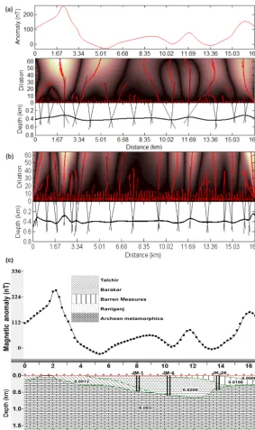
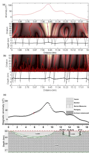
Jharia coalfield and surrounding areas have been consid-ered to estimate the source depths on the basis of technique of intersections of modulus maxima lines of CWT. The mean depths of causative sources along the profile AA0_{(passes east} of the Khanudih and west of the Telmuchu and Bansjora re-gion through Amdih over the westernmost part of the Jharia coalfield, shown in Fig. 2) calculated from the CWT (Fig. 5a) and Daubechies’ wavelet method (Fig. 5b) vary from 0.2 to 0.45 km. Profile AA0shows that there is fault near the north-western part of the basin.

Magnetic field inclination, declination and azimuth angle (clockwise from true north) of this profile are 36.44,−0.11 and 268.48◦respectively. The anomaly about 77 nT between boreholes JM-4 and JK-26 has been observed because of a number of basic intrusive bodies belonging to Satpura cycle that exist over the area. Jharia coalfield consists of peridotites in the form of sills as well as dykes. Dolerite dykes are very common in the western part of this coalfield.

The central part shows a flat sedimentary region and the magnetic anomaly shows a high value on either side of the profile. Raniganj formation exists on the southern side whereas Talchir formation exists on the northern side of this profile. However, the Barren Measures and the Barakar for-mation lie between the Raniganj and the Talchir forfor-mations. There is an intrusion of Archean metamorphics in Talchir for-mation which appears as an outcrop over the surface near

Amdih (Fig. 5c). Some of the boreholes provide informa-tion about the metamorphics along this profile. The maxi-mum thickness of the sediment along this profile is observed to be about 0.8 km.

Boreholes JM-1, JM-4 and JK-26 are located close to this profile, which touches metamorphics at a depth of about 0.4, 0.55 and 0.3 km respectively. These boreholes are located west of Bansjora and Telmuchu. The depth to the basement obtained from magnetic data is nearly equal to the depth obtained from gravity data along these profiles (Singh and Singh, 2015).

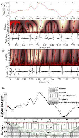
The mean depths of causative sources along the profile BB0(passes east of Telmuchu and Bansjora and west of Ku-mardih region, shown in Fig. 2) calculated from the CWT (Fig. 6a) and Daubechies’ wavelet (Fig. 6b) vary from 1.3 to 2.5 km. The central part of the basin shows the abrupt changes in the magnetic anomaly.

Profile BB0_{illustrates about the Barakar, Raniganj, Talchir} formations and Barren Measures. The Barren Measures is found between the Barakar and Raniganj formations and seen as an outcrop in both sides of the Raniganj formation. Also, an intrusion of the Talchir formation has been found in Archean metamorphics and an intrustion of the Barakar formation at the northern end of the profile (Fig. 6c). There is a sloppy nature of each formation below the profile from both ends. The major portion of this area is dominated by the Raniganj and the Barakar formations. The estimated thick-ness of the sediments is about 2.3 km over the Raniganj for-mation.

Magnetic field inclination, declination and azimuth angle of this profile are 36.42,−0.11 and 268.5◦respectively. This profile passes through two faults between metamorphics and sediment: one is at the southern end while the other is at the northern end of the profile. Faults are indicated by steep gra-dient of magnetic anomaly. The magnetic anomaly of about 103 and 162 nT southeast and east of Bansjora, respectively, represents the occurrence of Precambrian basement underly-ing the sediments.

The boreholes JK-7 and JM-8 are located near this pro-file. From borehole JM-7, it is obtained that maximum thick-ness of the Raniganj formation is about 0.22 km and Barren Measures lies below it. It touches the Barakar formation at a depth of about 1.2 km, east of Bansjora. From the obtained results from borehole JK-8, it is clear that sediment thickness is about 0.3 km and the borehole touches the Barren Mea-sures at a depth of about 300 m.

Figure 5. (a)Magnetic anomaly across the profile AA0(drawn in Fig. 2) and depth estimation by continuous wavelet transform.(b)Depth estimation by Daubechies’ wavelet method. (c)Geological section of the profile AA0 along with boreholes and magnetic susceptibility (shown in Table 2) of related formation.

the basin and the southern boundary is categorized by a more abrupt slope than the northern.

Magnetic field inclination, declination and azimuth an-gle of this profile are 36.41, −0.12 and 268.516◦ respec-tively. Gee (1932) mentioned four dykes in the memoir of this coalfield, namely Salama dyke, Sitarampur dyke, Cha-ranpur dyke and Barakar river dyke. The flow of the Barakar river is shown in Fig. 1. It is remarkable that in the region of this magnetic anomaly profile numbers of ultrabasic dyke

(mica peridotites) and sills are found as intrusive into sed-iments and Barakar formation causes magnetization of the body in the present earth’s field.

Figure 6. (a) Magnetic anomaly across the profile BB0and depth estimation by continuous wavelet transform.(b)Depth estimation by Daubechies’ wavelet.(c)Geological section of the profile BB0along with boreholes and magnetic susceptibility (shown in Table 2) of related formation.

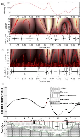
sections along the profile CC0 _{are also based on the results} obtained from gravity data (Singh and Singh, 2015), bore-hole information as well as geological information. Bore-holes NCJA-4, NCJA-5 and MN-11 are located near this pro-file. Boreholes NCJA-4 and NCJA-5 are located southwest of Katras and northeast of Kumardih. Depths of individual for-mations near the deepest part of the basin are about 0.4 km for Raniganj formation, 0.95 km for Barren Measures, 0.8 km for Barakar formation and 0.2 km for Talchir formation.

Figure 7. (a)Magnetic anomaly across the profile CC0(drawn in Fig. 2) and depth estimation by continuous wavelet transform.(b)Depth estimation by Daubechies’ wavelet.(c)Geological section of the profile CC0along with boreholes and magnetic susceptibility (shown in Table 2) of related formation.

Magnetic field inclination, declination and azimuth an-gle of this profile are 36.40, −0.12 and 268.529◦ respec-tively. Faults between Barakar formation and metamorphics are clearly indicated by steep gradients of magnetic anomaly at the northern end of the profile. The southern end of the profile is characterized by magnetic variation that appears to be due to an uneven topography. The middle of the profile is characterized by a magnetic high of about 151 nT because of 2-D linear features and a magnetic pole which lies nearly

0.5–0.65 km below the surface in this region. The extent of the Talchir formation assumed to be underlying the Barakar formation is uncertain. Some coal seams exhibited on the sur-face and northern side have a steeper dip than the southern side. Approximate depth of the basement in this area esti-mated from a single pole was 2 km (Fig. 8c) below the sur-face, southwest of Parbatpur.

Figure 8. (a)Magnetic anomaly across the profile DD0(drawn in Fig. 2) and depth estimation by continuous wavelet transform.(b)Depth estimation by Daubechies’ wavelet.(c)Geological section of the profile DD0along with boreholes and magnetic susceptibility (shown in Table 2) of related formation.

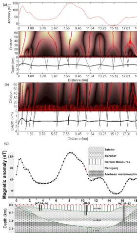
and geological information. Boreholes NCJA-14, JK-5 and NCJP-32 are located east of Katras, north west of Dubrajpur and west of Parbatpur respectively. The individual maximum thickness of various formations near the deepest part of the basin is about 0.8 km for Talchir, 0.4 km for Barren Measures and about 2 km for Barakar formation.

The mean depths of causative sources along the profile EE0 (passes east of the Parbatpur and Dubrajpur and west of Dungri, Kustore region, shown in Fig. 2) calculated from

the CWT (Fig. 9a) and Daubechies’ wavelet (Fig. 9b) vary from 1.8 to 2.8 km. There is a gentle slope of the basin on the northern side, uplift of the basement in the southern part and steep slope close to the southern boundary fault, clearly indicated in this profile.

Figure 9. (a)Magnetic anomaly across the profile EE0(drawn in Fig. 2) and depth estimation by continuous wavelet transform.(b)Depth estimation by Daubechies’ wavelet.(c)Geological section of the profile EE0 along with boreholes and magnetic susceptibility (shown in Table 2) of related formation.

surface. The anomaly high of about 149 nT at the middle of the profile could be ascribed to the presence of basic or ul-trabasic body which was a source for sills and basic dykes which intruded into the basin during Precambrian age. The south end of the underlying source is found to be at a depth of about 0.4 km and the north end at 0.7 km below the surface (Fig. 9c). The eastern margin shows the impact of the oc-currence of some faults and extension of metamorphic runs under the sediments up to a distance of about 1.12 km.

Geological sections along this profile are also deduced from the gravity data, borehole information and available

ge-ological information. Individual thickness of each formation is also deduced with the help of boreholes JK-4, NCJP-42, NCJP-16 and NCJP-12, which are located southwest of Ku-store, west of Nunikdih, west of Dungri and south of Dungri respectively. Maximum thickness is about 0.45 km for Barren Measures, 1.5 km for Talchir and 1.4 km for Barakar forma-tion.

Figure 10. (a)Magnetic anomaly across the profile FF0(drawn in Fig. 2) and depth estimation by continuous wavelet transform.(b)Depth estimation by Daubechies’ wavelet.(c)Geological section of the profile FF0along with boreholes and magnetic susceptibility (shown in Table 2) of related formation.

varies from 1 to 2.5 km. Also, magnetic anomaly suggests that this area is geologically highly disturbed and dips of the formations vary rapidly.

Magnetic field inclination, declination and azimuth angle of this profile are 36.33, −0.13 and 268.584◦ respectively. Patherdih horst, which is a tongue of gneiss, penetrates the southeast corner of this region. There are strong faults that occur at both ends of the profile. Several interesting

possibil-ities arise regarding the basic intrusives of dykes as well as schists which are normally magnetized. An anomaly of about 110 nT at the middle of the profile is due to peridotite dykes and sills having a close association with Barren Measures and Barakar formation.

Figure 11.The depth estimates obtained from Euler deconvolution (SI=2) are plotted in UTM coordinates of the study region.

Table 1.Mean depth of causative sources calculated from magnetic anomaly by CWT, EDM and Daubechies’ wavelet along the profiles drawn over Jharia coalfield and surrounding regions.

Distance and depth (km)

Depth at Depth at Depth at Depth at Depth at Depth at Depth at Names of 3 km from 6 km from 9 km from 12 km from 15 km from 18 km from 21 km from Profiles the left (km) the left (km) the left (km) the left (km) the left (km) the left (km) the left (km)

AA0 0.3 0.4 0.38 0.37 0.39 – –

BB0 2 2.4 2.2 2.5 1.8 – –

CC0 1.6 1.7 1.2 1.9 2 – –

DD0 2.2 2.8 1.7 1.8 2.3 – –

EE0 1.8 2.8 1.8 2 1.7 1.9 2.1

FF0 2.1 2.2 1 1.7 1.8 – –

dykes (mica peridotites) are found to be intrusive into the sediments. Geology over this profile could be ascribed to the presence of a basic or ultrabasic body which was the main source for the sills and basic dykes that intruded (Fig. 10c) into the basin during Gondwana times (Verma et al., 1973).

Geological strata along this profile are highly disturbed. Therefore, dips of the formations vary abruptly. The thick-ness of the formations is extrapolated from gravity data, boreholes NCJB-9, NCJB-25 and JFT-8 information as well as geological information. Boreholes NCJB-9, NCJB-25 and JFT-8 are located west of Chhatabad, west of Patherdih and west of Bhojudih respectively. Borehole JFT-8 has the cross contact between Barren Measures and Barakar formation and it touches the metamorphics about 0.4 km west of Bho-judih. The depth of the individual formations is approxi-mately equal to the depth obtained from interpretation of gravity data (Singh and Singh, 2015).

The interpretation of magnetic anomaly over Jharia coal-field has been compared with some information from inter-pretation of gravity data (Verma and Ghosh, 1974). The mean depth of the causative sources estimated by Euler deconvolu-tion method (Fig. 11) ranges about 0.6 to 3.2 km. The mean depth of the profiles has been shown in the Table 1.

Table 2.The following magnetic susceptibility used to prepare the geological sections. Susceptibility values are taken from the standard chart compiled by Clark and Emerson (1991) and Hunt et al. (1995).

Formation Litho-type Maximum volume Magnetic susceptibility (SI units)

Raniganj Fine-grained feldspathic sandstones, shales with coal seams

Sandstone=0.0209 Shale=0.0186 Coal=0.000025 Barren

Measures

Buff-colored sandstones, shales and carbonaceous shales

Sandstone=0.0209 Shale=0.0186

Barakar Buff-colored coarse and medium-grained feldspathic sandstones, car-bonaceous shales, fire clays and coal seams

Sandstone=0.0209 Shale=0.0186 Clay=0.00025 Coal=0.000025 Talchir Silt, carbonates

Greenish shale and fine-grained sandstones

Silt/carbonates=0.0012 Shale=0.0186 Sandstone=0.0209 Metamorphics Granite gneisses, quartzites, mica

schists and amphibolites

Granite=0.05 Gneisses=0.025 Quartzites=0.0044 Mica schists=0.003 Amphibolites=0.00075

Figure 11 shows two sets of fractures, predominantly ori-ented in the northeast and southeast at the northern and south-ern boundary respectively. The orientation of fractures sets are similar to that of the orientation obtained from regional magnetic interpretation (Verma et al., 1973). In the southern region, the depth of the Precambrian basement derived from the faults is less than that in the northern region. Furthermore, intense fracturing is detected at the center of the study area. In the western and southern regions, the basement depth is shallower compared to that of the eastern and northern re-gion.

Profile analysis suggests that most of the basement lies below 700 m, which is reasonable as calculated by wavelet transform method. The faults and depths obtained from the Euler deconvolution, CWT and Daubechies’ wavelet are re-lated to each other according to the results obtained from the regional magnetic interpretation.

7 Conclusions

The present analysis demonstrates the efficiency of continu-ous wavelet transform to delineate the locations of causative sources of potential field. Mean depth of the causative source along the profile AA0from across Amdih and south of Tel-muchu varies from 0.2 to 0.45 km and there is a fault near the northwestern part of the study region. The magnetic anomaly of about 77 nT corresponds to the number of basic intrusive bodies belonging to the Satpura cycle. Mean depth of the

8 Data availability

The data used in this paper can be found in the online Sup-plement for this article.

The Supplement related to this article is available online at doi:10.5194/gi-6-53-2017-supplement.

Competing interests. The authors declare that they have no conflict of interest.

Acknowledgements. Authors are very thankful to D. C. Panigrahi, Director of IIT (ISM) Dhanbad, for providing the necessary infrastructure for this research to be successfully carried out. We are very grateful to Lev Eppelbaum, Associate Editor of this journal, who gave the initial reviews on earlier versions of the manuscript that greatly improved the final paper. We would also like to show our gratitude to Sanjay Prajapati, O. Menshov and an anonymous reviewer for their positive comments.

Edited by: L. Eppelbaum

Reviewed by: S. K. Prajapati, O. Menshov, and one anonymous referee

References

Ardestani, E. V.: Precise Edge detection of gravity anomalies by Tilt angle filters, J. Earth & Space Phys., 36, 2, 11–19, 2010. Barbosa, V. C. F., Silva, J. B. C., and Medeiros, W. E.: Stability

analysis and improvement of structural index estimation in Euler deconvolution, Geophysics, 64, 48–60, 1999.

Blakely, R. J. and Simpson, R. W.: Approximating edges of source bodies from magnetic or gravity anomalies, Geophysics, 51, 1494–1498, 1986.

Bhattacharyya, B. P.: Tectono-metamorphic effect of granite and pegmatite emplacement in the Precambrian of Bihar Mica Belt. Proc. Symp. On Metallogeny of the Precambrian, Geological So-ciety of India, Bangalore, India, 45–56, 1972.

Coleman, T. F. and Li, Y.: An interior, trust region approach for nonlinear minimization subject to bounds, SIAM J. Optimiz., 6, 418–445, 1996.

Dewangan, P., Ramprasad, T., Ramana, M. V., Desa, M., and Shailaja, B.: Automatic interpretation of magnetic data using Eu-ler deconvolution with nonlinear background, Pure Appl. Geo-phys., 164, 2359–2372, 2007.

FitzGerald, D., Reid A., and McInerney, P.: New discrimination techniques for Euler deconvolution, Computat. Geosci., 30, 461– 469, 2004.

Fox, C. S.: The Jharia Coal Field, Geological Survey of India, Mem-oir, 56, 1–255, 1930.

Gee, E. R.: The geology and coal resources of the Raniganj coal-field, Mem. Geol. Surv. India, 61, 1–343, 1932.

Gerovska, D. and Arauzo Bravo, M. J.: Automatic interpretation of magnetic data based on Euler deconvolution with unprescribed structural index, Computat. Geosci., 29, 949–960, 2003. Goyal., P. and Tiwari, V. M.: Application of the continuous wavelet

transform of gravity and magnetic data to estimate sub-basalt sediment thickness, Geophys. Prospect., 62, 148–157, 2014. Gunn, P. J.: Linear transformations of gravity and magnetic fields,

Geophys. Prospect., 23, 300–312, 1975.

Holschneider, M., Chambodut, A., and Mandea, M.: From global to regional analysis of the magnetic field on the sphere using wavelet frames, Phys. Earth Planet. In., 135, 107–124, 2003. Hunt, C. P., Moskowitz, B. M., and Banerjee, S. K.: Magnetic

prop-erties of Rocks and Minerals, in: Rock Physics and Phase Rela-tions – A hand book of Physical constants, AGU Reference shelf 3, edited by: Ahrens, T. J., 189–204, 1995.

Hsu, S. K.: Imaging magnetic sources using Euler’s equation, Geo-phys. Prospect., 50, 15–25, 2002.

Hsu, S. K., Sibuet, J. C., and Shyu, C. T.: High resolution detec-tion of geologic boundaries from potential-field anomalies: an enhanced analytic signal: technique, Geophysics, 61, 373–386, 1996.

Keating, P. B.: Weighted Euler deconvolution of gravity data, Geo-physics, 63, 1595–1603, 1998.

Kopal., Z.: Numerical analysis, Chapman and Hall Ltd., London, UK, 551–553, 1961.

Moreau, F., Gibert, D., Holschneider, M., and Saracco, G.: Wavelet analysis of potential fields, Inverse Probl., 13, 165–178, 1997. Moreau, F., Gibert, D., Holschneider, M., and Saracco, G.:

Iden-tification of sources of potential fields with continuous wavelet transform: Basic theory, J. Geophys. Res., 104, 5003–5013, 1999.

Mushayandebvu, M. F., Van Driel, P., Reid, A. B., and Fairhead, J. D.: Magnetic source parameters of two dimensional structures using extended Euler deconvolution, Geophysics, 66, 814–823, 2001.

Mushayandebvu, M. F., Lesur, V., Reid, A. B., and Fairhead, J. D.: Grid Euler deconvolution with constraints for 2-D structures, Geophysics, 69, 489–496, 2004.

Perez, C., Wijns, C., and Kowalczyk, P.: Theta map: Edge detection in magnetic data, Geophysics, 70, L39–L43, 2005.

Ravat, D.: Analysis of the Euler method and its applicability in en-vironmental investigations, J. Environ. Eng. Geoph., 1, 229–238, 1996.

Reid, A. B., Allsop, J. M., Granser, H., Millet, A. J., and Somerton, I. W.: Magnetic interpretation in three dimensions using Euler deconvolution, Geophysics, 55, 80–91, 1990.

Reid, A. B., Ebbing, J., and Webb, S. J.: Avoidable Euler Errors- the use and abuse of Euler deconvolution applied to potential field, Geophys. Prospect., 62, 1162–1168, 2014.

Sailhac, P., Gibert, D., and Boukerbout, H.: The theory of the con-tinuous wavelet transform in the interpretation of potential fields: A review, Geophys. Prospect., 57, 517–525, 2009.

Salem, A., Williams, S., Fairhead, J. D., Ravat, D., and Smith, R.: Tilt-depth method: a simple depth estimation method using first order magnetic derivatives, The Leading Edge, 26/12, 1502– 1505, 2007.

Silva, J. B. C. and Barbosa, V. C. F.: 3-D Euler deconvolution: The-oretical basis for automatically selecting good solutions, Geo-physics, 68, 1962–1968, 2003.

Silva, J. B. C., Barbosa, V. C. F., and Medeiros, W. E.: Scattering, symmetry, and bias analysis of source position estimates in Eu-ler deconvolution and its practical implications, Geophysics, 66, 1149–1156, 2001.

Singh, A. and Singh, U. K.: Wavelet analysis of residual gravity anomaly profiles: Modeling of Jharia coal basin, India, 86, 679– 686, 2015.

Stavrev, P. and Reid, A.: Degrees of homogeneity of potential fields and structural indices of Euler deconvolution, Geophysics, 72, L1–L12, 2007.

Stavrev, P. Y.: Euler deconvolution using di?erential similarity transformations of gravity or magnetic anomalies, Geophys. Prospect., 45, 207–246, 1997.

Thompson, D. T.: EULDPH: A new technique for making com-puter assisted depth estimates from magnetic data, Geophysics, 47, 31–37, 1982.

Verma, R. K. and Ghosh, D.: Gravity survey over Jharia coalfield, India. Geophys. Res. Bull., 12, 165–175, 1974.

Verma, R. K., Prasad, S. N., and Jha, B. P.: Magnetic Survey over Jharia Coal Field, Pure Appl. Geophys., 102, 124–133, 1973. Verma, R. K., Majumdar, R., Ghosh, D., Ghosh, A., and Gupta,

N. C.: Results of Gravity Survey over Raniganj Coalfield, India, Geophys. Prospect., 24, 19–30, 1976.

Verma, R. K., Bhuin, N. C., and Mukhopadhyay, M.: Geology, Structure and tectonics of Jharia Coal Field, India-A 3-D Model, Geoexploration, 17, 305–324, 1979.

Williams, S., Fairhead, J. D., and Flanagan, G.: Grid based Euler deconvolution: Completing the circle with 2-D constrained Eu-ler, SEG Technical Program Expanded Abstracts, 22, 576–579, 2003.