MULTI-OBJECTIVE OPTIMAL REACTIVE POWER DISPATCH USING DIFFERENTIAL EVOLUTION

Http://www.ijetmr.com©International Journal of Engineering Technologies and Management Research [27]

MULTI-OBJECTIVE OPTIMAL REACTIVE POWER DISPATCH USING

DIFFERENTIAL EVOLUTION

Ram Kishan Mahate *1_{, Himmat Singh} 2

*1, 2 _{Department of Electrical Engineering, Madhav Institute of Technology and Science Gwalior,}

India Abstract:

Reactive power optimization is a major concern in the operation and control of power systems. In this paper a new multi-objective differential evolution method is employed to optimize the reactive power dispatch problem. It is the mixed–integer non linear optimization problem with continuous and discrete control variables such as generator terminal voltages, tap position of transformers and reactive power sources. The optimal VAR dispatch problem is developed as a nonlinear constrained multi objective optimization problem where the real power loss and fuel cost are to be minimized at the same time. A conventional weighted sum method is inflicted to provide the decision maker with a example and accomplishable Pareto-optimal set. This method underlines non-dominated solutions and at the same time asserts diversity in the non-dominated solutions. Thus this technique treats the problem as a true multi-objective optimization problem. The performance of the suggested differential evolution approach has been tested on the standard test system IEEE 30-bus.

Keywords: Reactive Power Management; Differential Evolution Algorithm; Power Loss Minimization; Voltage Deviation, Pareto-Optimal Solutions.

Cite This Article: Ram Kishan Mahate, and Himmat Singh. (2019). “MULTI-OBJECTIVE OPTIMAL REACTIVE POWER DISPATCH USING DIFFERENTIAL EVOLUTION.”

International Journal of Engineering Technologies and Management Research, 6(2), 27-38. DOI: https://doi.org/10.29121/ijetmr.v6.i2.2019.353.

1. Introduction

Optimal reactive power expedition problem is one of the difficult optimization worries in power systems. The origins of the reactive power are the generators, synchronous condensers, capacitors, static compensators and tap changing transformers. The problem that has to be figured out in a reactive power optimization is to find out the optimal values of generator bus voltage magnitudes, transformer tap setting and the output of reactive power origins so as to minimize the transmission loss. In recent years, the problem of voltage stability and voltage collapse has become a major worry in power system designing and procedure.

Http://www.ijetmr.com©International Journal of Engineering Technologies and Management Research [28]

genetic algorithms have been proposed to solve the reactive power optimization problem [5]. Genetic algorithm is a random search technique based on the mechanics of natural selection. But in the recent research some insufficiencies are distinguished in the GA performance. This abasement in efficiency is apparent in applications with highly hypostasis objective functions i.e. where the parameters being optimized are extremely correlated. In addition, the untimely convergence of GA degrades its performance and reduces its search capability. In addition to this, these algorithms are found to take more time to reach the optimal result.

More recently, a new evolutionary computation technique, called differential evolution (DE) algorithm, has been proposed and introduced [6-7]. The algorithm is motivated by biological and sociological motivations and can take care of optimality on bumpy, discontinuous and multi modal surfaces. The DE has three main advantages: it can find near optimal solution apart from the initial parameter values, its convergence is fast and it uses not many number of control parameters. In addition, DE is simple in coding, effortless to use and it can handle integer and discrete optimization. The performance of the DE algorithm was equated by the different heuristic techniques. It is determined from that compression, the DE is considerably better than that of other process. Also it is determined that DE is robust; it is able to replicate the same results consistently over many trials. In addition, DE algorithm has been used to solve high dimensional function optimization [8]. It is found that, it has better functioning on a set of generally used bench mark function. Therefore, the DE algorithm seems to be a predicting advance for engineering optimization problem [9].

The traditional approach is to formulate this problem as a single objective optimization problem with constraints. In this approach, the objective may consist of a single term or it may consist of multiple terms [10].The multi objective VAR dispatch problem was converted to a single objective problem by linear compounding of different objectives as a weighted sum [11]. Contrariwise, the studies on evolutionary algorithms, over the past few years, have shown that these methods can be expeditiously used to wipe out most of the difficulties of classical methods [12-13]. Since they use a population of solutions in their search, multiple Pareto-optimal solutions can, in principle, be found in one single run. The multi objective evolutionary algorithms have been carried out to environmental/economic power bump off problem with telling achiever.

The goal of this paper is to develop the RPD problem as a multi-objective optimization and exemplify its solution using Pareto based multi-objective optimization Differential evolution. Two different multi-objective problem formulations are provided.

Http://www.ijetmr.com©International Journal of Engineering Technologies and Management Research [29] 2. Problem Formulation

The optimal VAR management problem is to optimize the steady state performance of a power system in terms of one or more objective functions while satisfying several equality and inequality constraints. Generally the problem can be formulated as follows.

2.1.Objective Functions

Real power loss (PL)

This objective is to minimize the real power loss in transmission lines of the power system and is expressed as



k V V VV

g Ploss f 1 2 2

1 [ 2 cos(  )] (1)

where nl is the number of transmission lines; gk is the conductance of the kth line; and

are the voltages at the end buses i and j of the kth _{line, respectively.}

Fuel Cost Minimization

The objective of the ELD is to minimize the total system cost by adjusting the power output of each of the generators connected to the grid. The total system cost is modeled as the sum of the cost function of each generator (1). The generator cost curves are modeled with smooth quadratic functions, given by:

𝑓 ₂ = F_cost = ∑ a_i+ b_iP_Gi+ c_iP_Gi2 ($ h⁄ )

NG

i=1

(2)

Where NG is the number of online thermal units, PGi is the active power generation at unit i and

ai, bi and ci are the cost coefficients of the ith generator

2.2.Problem Constraints

Equality Constraints

The equality constraints represent typical load flow equations as follows



Gi P V V G B

P 1 0 )] sin( ) cos( [     (3)

sin( ) cos( ) 0

1 =  −  +  −  − −



= ij i j ij i j NB

j j i Di

Gi Q V V G B

Q

(4)

for i=1,...NB

i i V

Http://www.ijetmr.com©International Journal of Engineering Technologies and Management Research [30]

where NB is the number of buses; PG and QG are the generator real and reactive power, respectively; PD and QD are the load real and reactive power, respectively; Gijand Bij are the transfer conductance and susceptance between bus i and bus j, respectively.

Inequality Constraints

The inequality constraints represent the system operating constraints as follows.

Generation Constraints: Generator voltages VG and reactive power outputs QGare restricted by

their lower and upper limits as follows:

. ,..., 2 , 1 ,

max min

NG i

V V

V_Gi  _Gi _Gi =

(5)

NG i

Q Q

Q_Gimin  _Gi  _Gimax, =1...

(6)

where NG is the number of generators.

Transformer constraints: Transformer tap T settings are bounded as follows:

Ti Ti Ti ,i 1...NT

max

min  =

(7) where NT is the number of transformers.

Switchable VAR sources constraints: Switchable VAR compensations QC are restricted by their

limits as follows

NC i

Q Q

Q_cimin  _ci  _cimax, =1...

(8)

where NC is the number of switchable VAR sources.

Security constraints: These include the constraints of voltages at load buses VL and transmission

line loadings SL as follows:

. ... 1 ,

max min

NL i

V V

V_Li  _Li  _Li =

(9)

nl i

S

Sli li , 1...

max =



(10)

Aggregating the objectives and constraints, the problem can be mathematically formulated as a nonlinear constrained multi-objective optimization problem as follows.

Minimize [PL(x,u), VD(x,u)] (11)

Subject to;

Http://www.ijetmr.com©International Journal of Engineering Technologies and Management Research [31] h(x,u) = 0 (13)

where x is the vector of dependent variables consisting of load bus voltages VL, generator reactive power outputs QG, and transmission line loadings SL. Hence, x can be expressed as

xT _{= [V}

L1….VNL, QG1….QGNG, Sl1....Slnl] (14)

u is the vector of control variables consisting of generator voltages VG transformer tap settings T, and shunt VAR compensations Qc. Hence, u can be expressed as

uT _{= [V}

G1…. VGNG, T1….TNT, QC1….QCNC] (15)

Differential Evolution algorithm has been applied for this multi-objective reactive power management problem. This RPM problem is a combinatorial optimization problem with multi-extremism and non-linear property. To overcome the difficulties, the optimization variables, namely generator voltages and transformer tap-settings are considered as continuous values in this paper.

3. Multi-Objective Optimization

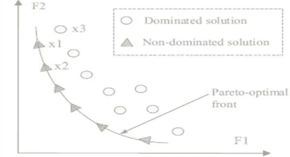
In many practical problems, several optimization criteria need to be satisfied simultaneously [15]. Moreover, it is often not advisable to combine them into a single objective. While it may sometimes happen that a single solution optimizes all of the criteria, the more likely scenario is when one solution is optimal with respect to a single criterion while other solutions are best with respect to the other criteria. The increase of the “goodness” of the solution with respect to one objective will produce a decrease of its “goodness” with respect to the others. While there are no problems in understanding the notion of optimality in single objective problems, multi objective optimization requires the concept of Pareto-optimality.

Figure 1: Pareto-optimality, non dominated and dominated solutions

Http://www.ijetmr.com©International Journal of Engineering Technologies and Management Research [32] Minimize F =[f1., f2] (16)

Subject to the constraints (3) – (10)

For a multi-objective optimization problem, any two solutions x1 and x2 _{can have one of two}

possibilities - one covers or dominates the other or none dominates the other. In a minimization problem, without loss of generality, a solution x1 dominates x2 if the following two conditions are

satisfied

) ( ) ( : } 2 , 1

{ f x₁ f x₂

i _i  _i

 (17)

) ( ) ( : } 2 , 1

{ f x₁ f x₂

j _j  _j



(18)

If any of the above conditions is violated, the solution x1 does not dominate the solution x2. If x1

dominates the solution x2, x1 is called the dominated solution. The solutions that are

non-dominated within the entire search space are denoted as optimal and constitute the Pareto-optimal set or Pareto-Pareto-optimal front. The Pareto-Pareto-optimal front depicts the Pareto-optimal tradeoffs that exist between the competing objectives. There are different approaches to solve multi-objective optimization problems like aggregating, population based non-Pareto, and Pareto based techniques. In aggregating technique, the different objectives are generally combined into one using weighing or goal-based method.

The present paper implements aggregating technique for solving the multi-objective RPM problem. The RPM problem has been treated as a single objective optimization problem by linear combination of PL and VD objectives as follows:

Minimize w×PL + (1-w) × fuel cost (19)

Where w is a weighing factor. For example to generate 20 non-dominated solutions, the algorithm has been applied 20 times with varying weighing factor w which is a random number rand [0,1], a uniformly distributed random number between 0 and 1.

4. Differential Evolution Algorithm

Http://www.ijetmr.com©International Journal of Engineering Technologies and Management Research [33]

Initialization

At the beginning of DE algorithm implementation, i.e. at t = 0, the problem independent variables are initialized somewhere in their feasible numerical range. Therefore, if the ith _{variable has its} lower and upper bounds as 𝑥_𝑖𝑙 and 𝑥_𝑖𝑢, respectively, then

the jth _{component of the i}th _{population member may be initialized as:}

) (

) 1 , 0 ( )

0

( l

j u j l

j

ij x rand x x

x = +  − (20)

where rand (0, 1) is a uniformly distributed random number between 0 and 1.

Mutation

In each generation, a donor vector vi(t) is created in order to change the population member vector

xi(t). Generally, the method of creating this donor vector is different in various DE schemes. However, in this paper, DE/rand/1 mutation strategy is implemented. In this mutation strategy, creation of the donor vector vi(t) for the ith member xi, three parameter vectors xr1, xr2and xr3, are selected randomly from the current population and not coinciding with the current member xi.

Next, a scalar number F scales the difference between any two of the three vectors and this scaled difference is added to the third one. Thus, the donor vector vi(t) is obtained. The jth component of

each vector can be expressed as:

) ( )

( ( ) ( )

1

( _{1, 2, 3,}

, t x t F x t x t

v_{i j} + = _{r j} + _{r j} − _{r j} (21)

Crossover

To increase the diversity of the population, crossover operator is carried out in which the donor vector exchanges its components with those of the current member xi(t). Two types of crossover schemes can be used by DE algorithm. These are exponential crossover and binomial crossover. Although the exponential crossover was presented in the original work of Storn and Price [3],the binomial variant is much more used in recent applications [7]. On the other hand, for the same value of CR, the exponential variant needs a larger value for the scaling parameter F in order to avoid premature convergence [1]. In this paper, binomial crossover scheme is used which is performed on all the D variables and can be expressed as:

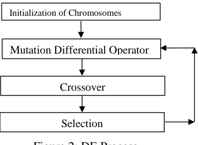
Initialization of Chromosomes

Figure 2: DE Process cycle

Mutation Differential Operator

Http://www.ijetmr.com©International Journal of Engineering Technologies and Management Research [34]      = else t x CR rand if t v t u j i j i j i ) ( ) 1 , 0 ( ) ( ) ( , , , (22) Selection

To keep the population size constant over subsequent generations, the selection process is applied to find out which one of the child and the parent will survive in the next generation, i.e. at time t =

t + 1. DE actually adopts the survival of the fittest principle in its selection process. The selection process can be expressed as,

( ) ( )

( ) ( )

Where f(.) is the function to be minimized. So, if the child Ui(t)

→

yields a better value of the fitness

function, it replaces its parent in the next generation; otherwise, the parent Xi(t)

→

is retained in the population. Thus, the population either gets better in terms of the fitness function or remains fixed but never degenerates. Hence, the population either gets better in terms of the fitness function or remains constant but never deteriorates.

5. Flow Chart and Steps Followed in DE Algorithm

Computational Steps of DE Algorithm

DE is utilized to find the best control variable setting starting from randomly generated initial population. At the end of each generation, the best individuals, based on the fitness value, are stored [8]. The detail of the proposed DE algorithm is as follows:

1) Generate an initial population randomly within the control variable bounds.

2) For each individual in the population, run load flow program such as NR method, to find the operating points.

3) Evaluate the fitness of the individuals. 4) Perform mutation and crossover operation 5) Select the individuals for the next generation 6) Store the best individual of the current generation. 7) Repeat steps ii–v, till the termination criterion is met.

8) Select the control variable setting corresponding to the overall best individual.

If the solution is acceptable, output the best individual and its objective value. Otherwise, take the settings corresponding to the next best individual and repeat the Step viii.

6. Results and Discussion

Http://www.ijetmr.com©International Journal of Engineering Technologies and Management Research [35]

magnitude limits at all buses are 0.95 pu and the upper limits are 1.1 pu for generator buses and 1.05 pu for the remaining buses. The lower and upper limits of the transformer tapings are 0.9 and 1.1 pu, respectively. Subsequently, the problem was handled as a multi-objective optimization problem where both power loss PL and Fuel cost were optimized simultaneously by converting it

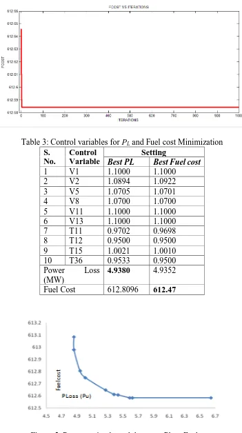
into a single objective optimization problem by linear combination of PL and Fuel cost objectives using (19). The DE algorithm was applied 41 times with varying weighing factor w generated randomly in the range of 0 to 1. The non-dominated solutions were selected by removing the inferior solutions from the total set of solution. Thus the Pareto-optimal set obtained has 12 non-dominated solutions and is shown in Fig. 3. Out of them, two non-non-dominated solutions that represent the best PL and best Fuel cost are given in Table 1. In this paper, the following values of DE key parameters are selected for the simultaneous optimization of the real power loss (PL) and

Fuel cost.

F = 0.2, CR = 0.8, NP = 15, GEN = 1000

Figure 3: Single line diagram of IEEE-30 bus system

Case1: Minimization of system power losses.

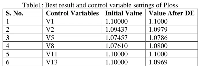
In this first case we run the algorithm for the minimization of power loss as a main objective function. The real power setting of the generator is taken from [12]. Table 1 shows the best result of Ploss function minimization.

Table1: Best result and control variable settings of Ploss

S. No. Control Variables Initial Value Value After DE

1 V1 1.10000 1.1000

2 V2 1.09437 1.0979

3 V5 1.07457 1.0786

4 V8 1.07610 1.0800

5 V11 1.10000 1.1000

Http://www.ijetmr.com©International Journal of Engineering Technologies and Management Research [36]

7 T11 1.06718 1.1000

8 T12 0.9000 0.9500

9 T15 1.04797 1.0924

10 T36 0.98354 1.000

Ploss (MW) 5.84230 4.5653

Fuel Cost 613.0778

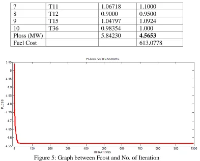
Figure 5: Graph between Fcost and No. of Iteration

Case 2: Minimization of system Fuel cost.

In this second case we run the algorithm for the minimization of fuel cost as a main objective function. The real power setting of the generator is taken from [12]. Table 2 shows the best result of fuel cost function minimization.

Table 2: Best result and control variable settings of Fuel cost

S. No. Control Variables Initial Value Value After DE

1 V1 1.10000 1.0770

2 V2 1.09437 1.0800

3 V5 1.07457 1.0492

4 V8 1.07610 1.0067

5 V11 1.10000 0.9796

6 V13 1.10000 0.9800

7 T11 1.06718 0.9700

8 T12 0.9000 0.9500

9 T15 1.04797 1.0600

10 T36 0.98354 1.1000

Ploss (MW) 5.8423 6.2182

Http://www.ijetmr.com©International Journal of Engineering Technologies and Management Research [37]

Table 3: Control variables for PL and Fuel cost Minimization

S. No.

Control Variable

Setting

Best PL Best Fuel cost

1 V1 1.1000 1.1000

2 V2 1.0894 1.0922

3 V5 1.0705 1.0701

4 V8 1.0700 1.0700

5 V11 1.1000 1.1000

6 V13 1.1000 1.1000

7 T11 0.9702 0.9698

8 T12 0.9500 0.9500

9 T15 1.0021 1.0010

10 T36 0.9533 0.9500

Power Loss

(MW)

4.9380 4.9352

Fuel Cost 612.8096 612.47

Http://www.ijetmr.com©International Journal of Engineering Technologies and Management Research [38] 7. Conclusion

In this paper differential evolution algorithm has been proposed and successfully applied to solve the optimal power flow problem. In this paper for solving the optimal power flow problem we can consider two objective functions these are Ploss and fuel cost these two objectives considered as single as well as multi objective to shows the effectiveness of the proposed algorithm. The proposed approach has been tested on standard IEEE-30 bus system; the same can be implemented for large size power systems as well.

References

[1] Lee K Y, Paru Y M, “Oritz J L –A united approach to optimal real and reactive power dispatch”, IEEE Transactions on power Apparatus and systems 1985: PAS-104 : 1147-1153

[2] A.Monticelli , M .V.F “Pereira ,and S. Granville , “Security constrained optimal power flow with post contingency corrective rescheduling” , IEEE Transactions on Power Systems :PWRS-2, No. 1, pp.175 182.,1987.

[3] Deeb N, Shahidehpur S.M, “Linear reactive power optimization in a large power network using the decomposition approach”. IEEE Transactions on power system 1990: 5(2) : 428-435

[4] D. Devaraj, and B. Yeganarayana, “Genetic algorithm based optimal power flow for security

enhancement”, IEE proc Generation. Transmission and. Distribution; 152, 6 November 2005 [5] Kwang Y. Lee and Frank F.Yang, “Optimal Reactive Power Planning Using evolutionary

Algorithms: A Comparative study for Evolutionary Strategy, Genetic Algorithm and Linear Programming”,IEEE Trans. on Power Systems, Vol. 13, No. 1, pp. 101- 108, February 1998. [6] R. Storn, K. Price, “Differential evolution—a simple and efficient adaptive scheme for global

optimization over continuous spaces”, in: Technical Report TR-95-012, ICSI, 1995.

[7] R. Storn, K. Price,” Differential evolution, a simple and efficient heuristic strategy for global

optimization over continuous spaces”, Journal of Global Optimization 11 (1997) 341–359. [8] Zhenyu Yang, Ke Tang, Xin Yao,” Differential evolution for high-dimensional function

optimization”, in IEEE Congress on Evolutionary Computation (CEC2007), 2007, pp. 3523–3530. [9] R. Balamurugan, S, Subramanaian, “Self-adaptive differential evolution based power economic dispatch of generators with valve-point effects and multiple fuel options”, Comput. Sci. Eng 1 (1) (2007) 10-17.

[10] N. Srinivas, K. Deb: “Multi-objective Optimization using Nondominated Sorting in Genetic Algorithm”, Evolutionary Computation, Vol. 2, No. 3, 1994, pp. 221-248.

[11] N. Grudinin, "Reactive Power Optimization Using Successive Quadratic Programming Method," IEEETrans. on PWRS, Vol. 13, No. 4, 1998, pp. 1219-1225.

[12] C. M. Fonseca and P. J. Fleming, “An Overview of Evolutionary Algorithms in Multiobjective

Optimization,” Evolutionary Computation, Vol. 3, No. 1, 1995, pp. 1-16.

[13] E. Zitzler and L. Thiele, “An Evolutionary Algorithm for Multiobjective optimization: The Strength

Pareto Approach,” Swiss Federal Institute of Technology, TIK-Report, No. 43, 1998.

[14] M.A. Abido,” Optimal power flow using particle swarm optimization”, Electric Power Energy Syst. 24 (7) (2002) 563–571.

[15] Miroslav M. Begovic, Branislav Radibratovic, Frank C Lambert, “On Multi objective Volt-VAR Optimization in Power Systems”, the 37th Hawaii International Conference on System Sciences - 2004

*Corresponding author.