Chebyshev Galerkin method for integro-differential equations of the second kind

(1)

Chebyshev Galerkin method for

integro-diﬀerential equations of the

second kind

J. Biazar∗ and F. Salehi

Abstract

In this paper, we propose an eﬃcient implementation of the Chebyshev Galerkin method for first order Volterra and Fredholm integro-diﬀerential equations of the second kind. Some numerical examples are presented to show the accuracy of the method.

Keywords: Volterra integro-diﬀerential equations; Galerkin method; Cheby-shev polynomials.

1 Introduction

Integro-differential equations occur in various areas. These equations arise in mathematical modeling of many scientific phenomena, such as fluid dy-namics, solid state physics, plasma physics, mathematical biology viscoelas-ticity [33], heat transfer [6], economics [26], chemostat [41], HIV models [4], biotissues [15], static analysis of wind towers or chimneys [35], and chemical kinetics [34]. Integro-differential equations contain both integral and differ-ential operators. The derivatives of the unknown functions may appear to any order [2, 40].

The concepts of integral equations have motivated a large amount of re-search work in recent years. Many numerical methods have been applied to solve these equations such as: El-gendi and Galerkin [11, 12, 27], Euler-Chebyshev [37], Variational iteration [39], Homotopy perturbation [10, 32], Chebyshev and Taylor collocation [1, 3, 8, 13, 20, 28], Chebyshev Wavelets [5],

∗_{Corresponding author}

Received 20 July 2014; revised 15 October 2014; accepted 1 July 2015 J. Biazar

Department of Applied Mathematics, Faculty of Mathematical Science, University of Guilan, Rasht, Iran. e-mail: [email protected]

F. Salehi

Department of Mathematics, Darab Branch, Islamic Azad University, Darab, Iran. e-mail: [email protected]

(2)

32 J. Biazar and F. Salehi

Spline collocation [7], finite element [9], sinc collocation [43], Bessel polynomi-als [42], Legendre polynomipolynomi-als [23], Bernstein polynomipolynomi-als [21] and Lagrange polynomials [31] and etc. [27, 36].

Galerkin method is a powerful tool for solving many kinds of equations in various fields of science and engineering. It is one of the most impor-tant weighted residual methods invented by the Russian mathematician Boris Grigoryevich Galerkin. Recently, various Galerkin algorithms have been ap-plied in numerical solution of integral equations and integro differential equa-tions. We can mention the following methods that are based on the Galerkin idea: Galerkin finite element [22], iterated Galerkin [38], Galerkin with hy-brid functions [27], Crank–Nicolson least–squares Galerkin [18], Wavelet– Galerkin [16], Discrete Galerkin [30], Petrov–Galerkin [25], pseudo–spectral Legendre–Galerkin [14] and etc. There are many different families of orthog-onal functions, which can be used. Chebyshev polynomials are considerably useful to solve integro-differential equations.

In this paper, the solution is approximated by a linear combination of the firstN+1 Chebyshev polynomials, with{ai}

N

i=0, as coeﬃcients. Approximate

solution will be simplified as a polynomial in x. This approximation will be substituted in the equation. To determineaj, one can consider inner product of both sides of the equation, byTj(x). This procedure reduces the problem to a system of equations. The generated system, which considering the type of the equation will be either linear or nonlinear, can be solved through various methods and the unknown coeﬃcients can be found. Practically, all orthogonal polynomials, on a closed finite interval, can also be applied for approximating functions. But convergence of the partial sums of the first-kind Chebyshev expansion, of a continuous function on [−1,1], is faster than the partial sums of an expansion in any other orthogonal polynomials [3].

The outline of this paper is as follows: Section 2 presents the method for solving Volterra integro-diﬀerential equations. Numerical examples are given in Section 3. Finally, conclusion will be presented in Section 4.

2 Chebyshev Galerkin method

Consider the following Volterra integro-diﬀerential equation

u′(x) =f(x) +λ

∫ x

a

K(x, t)u(t)dt , a≤x≤b, (1)

u(a) =α. (2)

where u(x) is the unknown function, K(x, t) is a known continuous and square integrable function, f(x) is a known function, andλis a real known parameter.

(3)

as a basis polynomial to approximate the solution on a closed finite interval. Assume that

u(x)≈uN(x) = N ∑

i=0

aiTi (

2x−(b−a)

b−a

)

, (3)

whereTi (

2x−(b−a)

b−a )

is shifted Chebyshev polynomial at [a, b]. So we have

u′(x)≈u′_N(x) = N ∑

i=0

2

b−aaiT

′ i

(

2x−(b−a)

b−a

)

. (4)

Substituting (3) and (4) into (1), results in N

∑

i=0

2

b−aaiT

′ i

(

2x−(b−a)

b−a

)

=f(x) +λ

n ∑ i=0 ai ∫ x a

K(x, t)Ti (

2t−(b−a)

b−a

)

dt, a≤x≤b. (5)

To determine unknown coeﬃcientsai, we use the Galerkin idea by multiplying both sides of (5) byTj

(

2x₋(b₋a)

b−a )

and then integrating with respect toxfrom

−1 to 1. So we have N

∑

i=0

2

b−aai

∫ 1

−1

T_i′

(

2x−(b−a)

b−a

)

Tj (

2x−(b−a)

b−a

)

dx= ∫ 1

−1

f(x)Tj (

2x−(b−a)

b−a

) dx+ ∫ 1 −1 ( λ n ∑ i=0 ai ∫ x a

K(x, t)Ti (

2t−(b−a)

b−a

)

dt

)

Tj (

2x−(b−a)

b−a

)

dx, (6)

forj= 0,1, . . . , N, or equivalently N

∑

i=0

2

b−aai

∫ 1

−1

T_i′

(

2x−(b−a)

b−a

)

Tj (

2x−(b−a)

b−a

)

dx= ∫ 1

−1

f(x)Tj (

2x−(b−a)

b−a

) dx+ λ n ∑ i=0 ai ∫ 1 −1 (∫ x a

K(x, t)Ti (

2t−(b−a)

b−a

)

dt

)

Tj (

2x−(b−a)

b−a

)

(4)

If needed the integrals can be calculated by numerical methods. This proce-dure generates a system of linear equations for the unknown {ai}

N

i=0. Many

researchers substitute initial condition

u(a) =α⇒

N ∑

i=0

aiTi (

2a−(b−a)

b−a

) =

N ∑

i=0

aiTi(−1) = α. (8)

for the same number of equations in the foregoing linear system.

The unknown parameters are determined by solving the system of equations (7) and (8). Substituting these values in (3) gives the approximate solution of the integro-diﬀerential equation (1). Similarly one can apply this approach for a Fredholm integro-diﬀerential equation in the following general form:

u′(x) =f(x) +λ

∫ b

a

K(x, t)u(t)dt , a≤x≤b, u(a) =α

3 Numerical Examples

In this section, we intend to show the eﬃciency of the Galerkin method for solving Volterra integro-diﬀerential equations of the second kind by Cheby-shev polynomials by presenting three illustrative examples. The absolute error for this formulation is defined by

E(x) =|u(x)−uN(x)|.

Example 1. Consider the following Fredholm integro-diﬀerential equations of the second kind [17]

u′(x) =u(x)−1 2x+

1

(x+ 1)−ln (x+ 1) + 1 (ln 2)2

∫ 1

0

x

t+ 1u(t)dt, (9)

u(0) = 0,

with the exact solutionu(x) = ln(x+ 1).

To solve Equation (9) we approximateu(x) andu′(x) as follows:

u4(x) = 4

∑

i=0

aiTi (

2x−(b−a)

b−a

)

=a0+a1(2x−1)

+a2(8x2−8x+ 1) +a3(32x3−48x2+ 18x−1)

(5)

and

u′₄(x) =

4

∑

i=0

2

b−aaiT

′ i

(

2x−(b−a)

b−a

)

= 2a1+a2(16x−8)

+a3(96x2−96x+ 18) +a4(512x3−768x2+ 320x−32). (11)

Substituting (10) and (11) into (9), results in

2a1+a2(16x−8) +a3(96x2−96x+ 18) +a4(512x3−768x2+ 320x−32)

=a0+a1(2x−1) +a2(8x2−8x+ 1) +a3(32x3−48x2+ 18x−1)

+a4(128x4−256x3+ 160x2−32x+ 1)−

1 2x+

1

(x+ 1)−ln (x+ 1)

+ x

(ln 2)2

∫ 1

0

1

t+ 1 (

a0+a1(2t−1) +a2(8t2−8t+ 1)

+a3(32t3−48t2+ 18t−1) +a4(128t4−256t3+ 160t2−32t+ 1)

)

dt,

(12) By multiplying both sides of (12) by Tj

(

2x₋(b₋a)

b−a )

and then integrating it with respect toxfrom−1 to 1, we obtain a system of linear equations which one of them is replaced by the equation

u(0) = 0⇒α0−α2+α4= 0 (13)

Now the unknown coeﬃcients {ai}

4

i=0 are determined by solving this

sys-tem. Substituting these values in (3) gives the approximate solution of the integro-diﬀerential equation (1). The results have been shown in Table 1, for

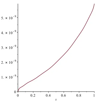
N = 4,8,12, and Error is plotted in Figure 1, forN = 12.

Example 2. Consider the following Volterra integro-diﬀerential equations of the second kind [40]

u′(x) = 1−2xsin (x) + ∫ x

0

u(t)dt, u(0) = 0.

The exact solution isy=xcos(x).

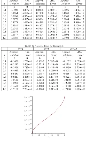
Table 2 shows the results forN= 4,8,12. Also Figure 2 shows absolute error forN = 12.

Example 3. Consider the following Volterra integro-diﬀerential equations [40]:

u′(x) =−1 + 1 2x

2₋_xex₋ ∫ x

0

(6)

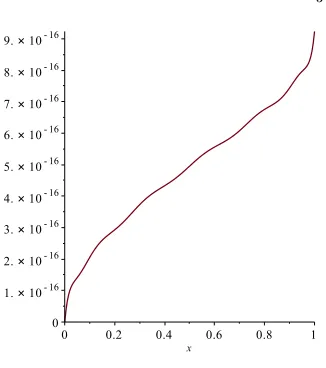
The exact solution is y = 1−ex_{. Results have been shown in Table 3, for}

N = 4,8,12, and Error plotted in Figure 3, forN = 12.

Table 1: Absolute Error for Example 1

N=4 N=8 N=12

Approx. Abs. Approx. Abs. Approx. Abs. x solution Error solution Error solution Error

0.0 0 0 0 0 0 0

0.1 0.0949 4.233e-4 0.0953 4.556e-7 0.0953 4.998e-10 0.2 0.1817 6.317e-4 0.1823 7.690e-7 0.1823 7.938e-10 0.3 0.2615 8.544e-4 0.2624 1.082e-6 0.2624 1.146e-09 0.4 0.3353 1.161e-3 0.3365 1.416e-6 0.3365 1.508e-09 0.5 0.4039 1.543e-3 0.4055 1.860e-6 0.4055 1.964e-09 0.6 0.4680 1.971e-3 0.4700 2.361e-6 0.4700 2.481e-09 0.7 0.5282 2.430e-3 0.5306 2.909e-6 0.5306 3.088e-09 0.8 0.5848 2.951e-3 0.5878 3.614e-6 0.5878 3.821e-09 0.9 0.6382 3.626e-3 0.6418 4.438e-6 0.6419 4.687e-09 1.0 0.6885 4.629e-3 0.6931 5.611e-6 0.6931 5.930e-09

(7)

N=4 N=8 N=12

0 0 0 0 0 0 0

0.1 0.0991 4.308e-4 0.0995 2.308e-9 0.0995 1.383e-15 0.2 0.1954 5.890e-4 0.1960 3.450e-9 0.1960 1.987e-15 0.3 0.2859 6.954e-4 0.2866 4.423e-9 0.2866 2.570e-15 0.4 0.3676 8.387e-4 0.3684 5.136e-9 0.3684 3.046e-15 0.5 0.4378 1.023e-3 0.4388 6.131e-9 0.4388 3.586e-15 0.6 0.4940 1.214e-3 0.4952 7.178e-9 0.4952 4.160e-15 0.7 0.5340 1.381e-3 0.5354 8.072e-9 0.5354 4.747e-15 0.8 0.5558 1.537e-3 0.5574 9.368e-9 0.5574 5.509e-15 0.9 0.5577 1.776e-3 0.5594 1.094e-8 0.5594 6.371e-15 1.0 0.5380 2.300e-3 0.5403 1.382e-8 0.5403 8.087e-15

N=4 N=8 N=12

0 0 0 0 0 0 0

0.1 -0.1050 1.750e-4 -0.1052 5.037e-10 -0.1052 2.053e-16 0.2 -0.2212 2.406e-4 -0.2214 7.428e-10 -0.2214 2.930e-16 0.3 -0.3496 2.785e-4 -0.3499 9.426e-10 -0.3499 3.730e-16 0.4 -0.4915 3.251e-4 -0.4918 1.069e-9 -0.4918 4.332e-16 0.5 -0.6483 3.850e-4 -0.6487 1.240e-9 -0.6487 4.955e-16 0.6 -0.8217 4.448e-4 -0.8221 1.407e-9 -0.8221 5.561e-16 0.7 -1.0130 4.891e-4 -1.0140 1.516e-9 -1.0140 6.081e-16 0.8 -1.2250 5.177e-4 -1.2260 1.679e-9 -1.2260 6.757e-16 0.9 -1.4590 5.648e-4 -1.4600 1.874e-9 -1.4600 7.438e-16 1.0 -1.7180 7.204e-4 -1.7180 2.311e-9 -1.7180 9.235e-16

(8)

Figure 3: Absolute Error for Example 3

4 Conclusion

This article deals with the numerical solution of the first order Volterra integro-diﬀerential equations of the second kind, using Galerkin method by Chebyshev Polynomials. This technique is tested on three examples and the results are satisfactory. In addition this method is portable to high order Volterra integro-diﬀerential equations of the second kind and easy to pro-gram.

Acknowledgment

Authors would like to thank anonymous reviewers for their valuable, useful, and constructive comments, that without their suggestion this paper was not competent enough to be published in this journal.

Authors also expressed their gratitude to the University of Guilan for financial support.

References

(9)

2. Atkinson, K.The Numerical Solution of Integral Equations of the Second Kind, Cambridge University Press, 1997.

3. Avazzadeh, Z. and Heydari, M.Chebyshev polynomials for solving two dimensional linear and nonlinear integral equations of the second kind, Comp. Appl. Math. 31(1) (2012), 127–142.

4. Banks, H., Bortz, D. and Holt, S.Incorporation of variability into the modeling of viral delays in HIV infection dynamics, Math. Biosci 183 (2003) 63-91.

5. Barzkar, A., Oshagh, M., Assari, P. and Mehrpouya, M.Numerical So-lution of the Nonlinear Fredholm Integral Equation and the Fredholm Integro-diﬀerential Equation of Second Kind using Chebyshev Wavelets, World Appl. Sci. J. 18(12) (2012) 1774-1782.

6. Boland, J. The analytic solution of the diﬀerential equations describing heat flow in houses, Build. Environ. 37(2002), 1027–1035.

7. Brunner, H.The approximate solution of initial-value problems for gen-eral Volterra integro-diﬀerential equations, Comput. 40(40) (1988) 125-137.

8. Cerdik-Yaslan, H. and Akyuz-Dascioglu, A. Chebyshev polynomial so-lution of nonlinear Fredholm-Volterra integro-diﬀerential equations, J. Arts. Sci. 5 (2006) 89-101.

9. Chen, C. and Shih ,T. Finite Element Methods for Integro diﬀerential Equations, Singapore: World Scienti?c Publishing Co Ltd, 1997.

10. Dehghan, M. and Shakeri, F. Solution Of An Integro-Diﬀerential Equa-tion Arising In Oscillating Magnetic Fields Using He’s Homotopy Per-turbation Method, Progr. In Electromagnetics Res., PIER 78 (2008) 361– 376.

11. Delves, L. and Mohamed, J.Computional Methods for Integral Equations, Cambridge: Cambridge University Press, 1985.

12. El-gendi, S. Chebyshev solution of diﬀerential, integral and integro- dif-ferential equations, Comput. J. 12 (1969) 282-287.

13. Ezzati, R. and Najafalizadeh, S. Numerical solution of nonlinear Volterra-Fredholm integral equation by using Chebyshev polynomials, Mathematical Sciences 5(1) (2011) 1-12.

(10)

15. Fung, B.Y.C.Mechanical Properties of Living Tissues, Springer-Verlag, New York, Springer-Verlag, New York, 1993.

16. Ghasemi, M., Tavassoli kajani, M. and Babolian, E.Numerical solutions of the nonlinear integro-diﬀerential equations: Wavelet-Galerkin method and homotopy perturbation method, Appl. Math. Comp. 188(1) (2007) 450-455.

17. Golbabai, A. and Seifollahi, S. Radial basis function networks in the numerical solution of linear integro-diﬀerential equations, Appl. Math. Comput. 188 (2007) 427–432.

18. Guo, H. and Rui, H. Crank–Nicolson least-squares Galerkin procedures for parabolic integro-diﬀerential equations, Appl. Math. Comp. 180 (2) (2006) 622-634.

19. Holmaker, K. Global asymptotic stability for a stationary solution of a system of integro-diﬀerential equations describing the formation of liver zones, SIAM J. Math. Anal. 24(1) (1993) 116–128.

20. Huang, Y. and Li, X. Approximate solution of a class of linear integro-diﬀerential equations by Taylor expansion method, Int. J. Comput. Math 15(3) (2009) 1–12.

21. Isik, O., Sezer, M. and Gney, Z. Bernstein series solution of a class of linear integro-diﬀerential equations with weakly singular kernel, Appl. Math,Comput. 217 (2011) 7009–7020.

22. Jangveladze, T., Kiguradze, Z. and Neta, B. Galerkin finite element method for one nonlinear integro-diﬀerential model, Appl. Math. Comp. 217(16) (2011) 6883-6892.

23. Khater, A., Shamardan, A., Callebaut, D. and Sakran, M.Numerical so-lutions of integral and integro-diﬀerential equations using Legendre poly-nomials, Numer. Alg. 46 (2007) 195–218.

24. Lewis, B.A.,On the numerical solution of Fredholm integral equations of the first kind, J. Inst. Math. Appl. 16(2) (1975) 207–220.

25. Lin, T., Lin, Y., Rao, M. and Zhang, S. Petrov-Galerkin Methods for Linear Volterra Integro-Diﬀerential Equations, SIAM J. Numer. Anal. 38(3) (2001) 937-963.

(11)

27. Maleknejad, K. and Tavassoli Kajani, M. Solving linear integro-diﬀerential equation system by Galerkin methods with hybrid functions, Appl. Math. Comput. 159 (2004) 603–612.

28. Maleknejad, K., Sohrabi, S. and Rostami, Y.Numerical solution of non-linear Volterra integral equation of the second kind by using Chebyshev polynomials, Appl. Math. Cmput. 188 (2007) 123-128.

29. Mason, J.C. and Handscomb, D. Chebyshev Polynomials, Boca Raton: Chapman & Hall/CRC, 2003.

30. Pedas, A. and Tamme, E.Discrete Galerkin method for Fredholm integro-diﬀerential equations with weakly singular kernels, Journal of Computa-tional and Applied Mathematics 213(1) (2008) 111-126.

31. Rashed, M.Lagrange interpolation to compute the numerical solutions of diﬀerential, integral and integro-diﬀerential equation, Appl. Math. Com-put. 151 (2004) 869–878.

32. Saberi-Nadjafi, J. and Ghorbani, A.He’s homotopy perturbation method: an eﬀective tool for solving nonlinear integral and integro-diﬀerential equations, Comput. Math. Appl. 58 (2009) 2379-2390.

33. Sergeev, V. On stability of viscoelastic plate equilibrium, Automat. Re-mote Control 68(9) (2007) 1544–1550.

34. Thieme, H.R. A model for the spatial spread of an epidemic, J. Math. Biol. 4 (1977) 337–351.

35. Tomasiello, S. A note on three numerical procedures to solve Volterra integro-diﬀerential equations in structural analysis, Comput. Math. Appl. 62(8) (2011) 3183–3193.

36. Tomasiello, S. Some remarks on a new DQ-based method for solving a class of Volterra integro-diﬀerential equations, Appl. Math. Comput. 219 (2012) 399–407.

37. Van der Houwen, P. and Sommeijer, B. Euler–Chebyshev methods for integro-diﬀerential equations, Appl. Numer. Math. 24 (1997) 203–218.

38. Volk, W. The iterated Galerkin method for linear integro-diﬀerential equations, J. Comp. Appl. Math. 21(1) (1988) 63-74.

39. Wang, S. and He, J. Variational iteration method for solving integro-diﬀerential equations, Physics letters A 367 (2007) 188–191.

(12)

41. Wolkowicz, G., Xia, H. and Ruan, S. Competition in the chemostat: a distributed delay model and its global asymptotic behavior, SIAM J. Appl. Math. 57 (1997) 1281–1310.

42. Y¨uzba¸sı, S., Sahidin, N. and Sezer, M. Bessel polynomial solutions of high-order linear Volterra integro-diﬀerential equations, Comput. Math. Appl 62(4) (2011) 1940–1956.

(13)

۲_{ﯽﺤﻟﺎﺻ هﺪﯾﺮﻓ و}۱_{رازآ ﯽﺑ ﺮﻔﻌﺟ}

ناﺮﯾا ،ﺖﺷر ،نﻼﯿﮔ هﺎﮕﺸﻧاد ،ﯽﺿﺎﯾر مﻮﻠﻋ هﺪﮑﺸﻧاد،ﯽﺿﺎﯾر هوﺮﮔ۱ ناﺮﯾا ،باراد ،ﯽﻣﻼﺳا دازآ هﺎﮕﺸﻧاد ،باراد ﺪﺣاو ،ﯽﺿﺎﯾر هوﺮﮔ۲

١٣٩۴ ﺮﯿﺗ ١٠ ﻪﻟﺎﻘﻣ شﺮﯾﺬﭘ ،١٣٩٣ ﺮﻬﻣ ٢٣ هﺪﺷ حﻼﺻا ﻪﻟﺎﻘﻣ ﺖﻓﺎﯾرد ،١٣٩٣ ﺮﯿﺗ ٢٩ ﻪﻟﺎﻘﻣ ﺖﻓﺎﯾرد

ﻪﺒﺗﺮﻣ ﻞﯿﺴﻧاﺮﻔﯾد-لاﺮﮕﺘﻧا تﻻدﺎﻌﻣ یاﺮﺑ ،ﻦﯿﮐﺮﻟﺎﮔ ﻒﺸﯿﺒﭼ شور زا ﺮﺛﻮﻣ یاﺮﺟا ﮏﯾ ،ﻪﻟﺎﻘﻣ ﻦﯾا رد: هﺪﯿﮑﭼ هﺪﺷ ﻪﺋارا شور ﺖﻗد نداد نﺎﺸﻧ یاﺮﺑ یدﺪﻋ لﺎﺜﻣ ﻦﯾﺪﻨﭼ .دﻮﺷ ﯽﻣ دﺎﻬﻨﺸﯿﭘ مود عﻮﻧ ﻢﻠﻫدﺮﻓ و اﺮﺘﻟو لوا .ﺖﺳا