Biorthogonal cubic Hermite spline multiwavelets on the interval for solving the fractional optimal control problems

Biorthogonal cubic Hermite spline multiwavelets on the interval for

solving the fractional optimal control problems

Elmira Ashpazzadeh

Department of Applied Mathematics, Faculty of Mathematical Sciences, University of Tabriz, Tabriz, Iran. E-mail: [email protected]

Mehrdad Lakestani∗

Department of Applied Mathematics, Faculty of Mathematical Sciences, University of Tabriz, Tabriz, Iran. E-mail: [email protected]

Abstract In this paper, a new numerical method for solving fractional optimal control problems (FOCPs) is presented. The fractional derivative in the dynamic system is described in the Caputo sense. The method is based upon biorthogonal cubic Hermite spline multiwavelets approximations. The properties of biorthogonal multiwavelets are first given. The operational matrix of fractional Riemann-Lioville integration and multi-plication are then utilized to reduce the given optimization problem to the system of algebraic equations. In order to save memory requirement and computational time, a threshold procedure is applied to obtain spare algebraic equations. Illustrative examples are provided to confirm the applicability of the new method.

Keywords. Caputo fractional derivative, Fractional order optimal control, Biorthogonal cubic Hermite spline multiwavelets.

2010 Mathematics Subject Classification. 65L05, 34K06, 34K28.

1. Introduction

In the present paper, we focus on optimal control problems with the quadratic performance index and the dynamic system with the Caputo fractional derivative as follows

M in J(x, u) =1 2

∫ t1

t0

[q(t)x2(t) +r(t)u2(t)]dt, (1.1)

C t0D

α

tx(t) =a(t)x(t) +b(t)u(t), (1.2)

x(t0) =x0, (1.3)

where q(t) ≥ 0, r(t) >0 and b(t) ̸= 0. The behavior of many real-world physical phenomena is governed by fractional differential equations (FDEs) [24]. FDEs are generalizations of ordinary differential equations to an arbitrary (non-integer) order.

Received: 4 August 2016 ; Accepted: 8 November 2016. ∗Corresponding author.

When these equations are used in conjunction with a performance index and a set of initial conditions, they lead to FOCPs. Fractional optimal control theory is a very new area in mathematics and the number of publications on this subject is limited.

Wavelet theory is a relatively new and an emerging area in mathematical research [20]. It has been applied in a wide range of engineering disciplines; particularly, wavelets are very successfully used in signal analysis for wave form representations and segmentations, time–frequency analysis and fast algorithms for easy implemen-tation [13]. Wavelets permit the accurate representation of a variety of functions and operators. Moreover, wavelets establish a connection with fast numerical algorithms [12].

The main aim of this paper is to employ biorthogonal cubic Hermite spline mul-tiwavelets on the interval [0,1] as the interpolating functions to achieve high perfor-mance computations of FOCPs. Our method consists of reducing the FOCP to a set of algebraic equations. We approximate the fractional state rateC_t0D_tαx(t) and con-trol variable u(t) with biorthogonal multiwavelets with unknown coefficients. Then the operational matrices of the Riemann–Liouville fractional integration and product are utilized to achieve a linear system of algebraic equation, instead of performance index (1.1) and dynamical system (1.2) in terms of unknown coefficients. Finally, the method of constrained extremum is applied which consists of adjoining the constraint equations derived from given dynamical system to the performance index by a set of undetermined Lagrange multipliers. As a result, the necessary conditions of opti-mality are derived as a system of algebraic equations in the unknown coefficients of

C t0D

α

tx(t) andu(t) and the Lagrange multipliers. These coefficients are determined in

such a way that the necessary conditions for extremization are imposed. Generally the use of biorthogonal cubic Hermite spline multiwavelets appears to be attractive since these functions possess several useful properties, such as small support, exact representation of polynomials to degree 3, Hermite interpolatory nature and the abil-ity to represent functions at different levels of resolution, these considerations reduce the computations. The main advantage of the new method is that with the use of threshold procedure for biorthogonal multiwavelets, we obtain spare algebraic equa-tion and this is computaequa-tionally very attractive and reduces CPU time.

Some numerical simulations for FOCPs with Riemann–Liouville fractional derivative can be found in [4,5, 11,22, 26]. Also there exist numerical simulations for FOCPs with the Caputo fractional derivative such as [6,7,27], where the author has solved the problem by solving the Hamiltonian equations approximately. Lotfi et. al. [22] and Keshavarz et. al [18] have solved the linear quadratic FOCP directly without using Hamiltonian formula. Also we refer the interested reader in fractional opti-mization problems to see [1,2,3,8,9,10,11,12,14,19,21,23] for some recent works in the subject.

with the numerical solutions obtained by [18, 22]. Finally, Section 6 completes this paper with a brief conclusion. Note that we have computed the numerical results by MAPLE programming.

2. _{Basic definition on fractional calculus}

We give some basic definitions and properties of the fractional calculus theory which are used further in this paper.

Definition 2.1. The Riemann–Liouville fractional integral of orderα >0 of a func-tionf is defined as follows [25]

0Itαf(t) =   

1 Γ(α)

∫t 0(t−τ)

α−1_{f(τ)dτ, α >0,}

f(t), α= 0.

Definition 2.2. The Caputo fractional derivative of order α >0 of a function f is defined as follows

C 0D

α tf(t) =

  

1 Γ(n−α)

∫t 0(t−τ)

n₋α₋1 d n

dτnf(τ)dτ, n−1< α < n,

f(n)_{(t), α=n.}

wherenis a positive integer.

For Riemann–Liouville fractional integration and the Caputo fractional derivative we have the following properties [25].

(1) For real values ofα >0, the Caputo fractional derivative provides the opera-tion inverse to the Riemann–Liouville integraopera-tion from the left

C 0D

α

t 0Itαf(t) =f(t), α >0, f(t)∈C[0,1]. (2.1)

(2) iff(t)∈C⌈α⌉_{[0,1], then}

0Itα C 0D

α

tf(t) =f(t)−

⌈α_∑⌉−1

j=0

tj

j!

(

dj

dtjf )

(0), n−1< α≤n, (2.2)

whereC⌈α⌉_{[0,1] is the space of⌈α⌉times continuously differentiable functions.}

3. Biorthogonal Hermite cubic spline multiwavelets

The widely used Hermite cubic splinesϕ= (ϕ1, ϕ2)Tare given by [16] ϕ1(x) := (1−3x2−2x3)χ[₋1,0]+ (1−3x2+ 2x3)χ[0,1],

ϕ2(x) := (x+ 2x2+x3)χ[−1,0]+ (x−2x2+x3)χ[0,1]. (3.1)

Note thatϕ∈(C1(R))2is a Hermite interpolant of order 1 satisfying

where δ is the Dirac sequence such that δ(0) = 1 and δ(k) = 0 for all k ∈Z\{0}. Moreover, the Hermite cubic spline vector-valued function ϕ is a refinable vector function satisfying

ϕ(x) = 2∑

k∈Z

a(k)ϕ(2x−k), x∈R, (3.3)

with the following matrix-valued mask:

a(−1) =

[ ₁ 4

3 8 −1

16 − 1 16

]

, a(0) =

[₁ 2 0

0 1₄

]

, a(1) =

[₁

4 −

3 8 1 16 −

1 16

]

(3.4)

anda(k) = 0 for allk∈Z\{−1,0,1}. Note thatϕ1and ϕ2 have symmetry: ϕ1(x) = ϕ1(−x) andϕ2(x) =−ϕ2(−x) for allx∈R.

Defineψ= (ψ1, ψ2)T as follows [17]

ψ1(x) =ϕ1(2x)−1₂(ϕ1(2x+ 1) +ϕ1(2x−1))−23₁₂(ϕ2(2x+ 1)−ϕ2(2x−1)), ψ2(x) =37₂₂ϕ2(2x) +91₈₈(ϕ2(2x+ 1) +ϕ2(2x−1)) +1₈(ϕ1(2x+ 1)−ϕ1(2x−1)).

(3.5)

Note that ϕ1_{, ϕ}2 _{and ψ}1_{, ψ}2 _{are supported inside [−1,1]. The functions ϕ}1_{, ψ}1 _are

symmetric about the origin, whileϕ2_{, ψ}2 _{are antisymmetric about the origin.}

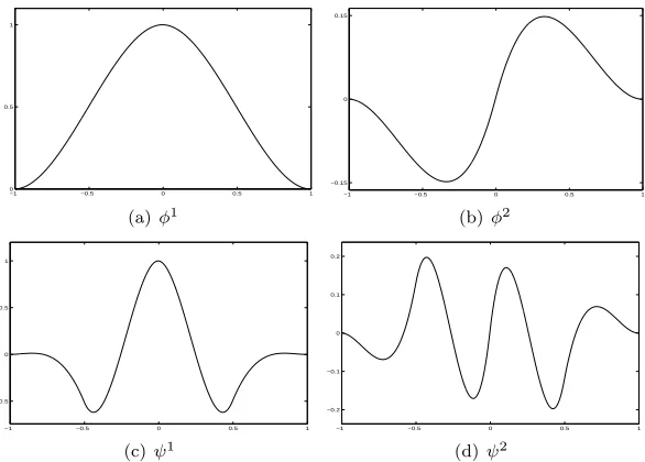
More-over, bothψ1_{, ψ}2_{have at least order 2 vanishing moments. See Figure 1 for the graphs}

of the refinable vector functionϕand wavelet vector functionψ.

Figure 1. The graphs of the biorthogonal wavelet ({ϕ;ψ}) forL2(R), where ϕ = (ϕ1_{, ϕ}2₎T_{is the spline Hermite refinable interpolant and ψ =}

(ψ1_{, ψ}2₎T_{is the wavelet vector function.}

−1 −0.5 0 0.5 1

0 0.5 1

(a)ϕ1

−1 −0.5 0 0.5 1

−0.15 0 0.15

(b)ϕ2

−1 −0.5 0 0.5 1

−0.5 0 0.5 1

(c)ψ1

−1 −0.5 0 0.5 1

−0.2 −0.1 0 0.1 0.2

3.1. Function Approximation. In this section we consider the approximation prop-erties of wavelet bases on the interval [0,1]. A Riesz wavelet basis BJ0,J = Φ⃗J0∪

∪J₋1 j=J0

⃗

Ψj forL2([0,1]) is given by

⃗ Φj =

[_√

2ϕ1₂j;0|[0,1], ϕ12j_;1, ϕ

2

2j_;1, . . . , ϕ

1

2j_;2j₋₁, ϕ

2 2j_;2j₋₁,

√

2ϕ1₂j_;2j|[0,1] ]T

, (3.6)

⃗ Ψj =

[_√

2ψ₂1j_;0|[0,1], ψ21j_;1, ψ

2

2j_;1, . . . , ψ

1

2j_;2j₋₁, ψ

2 2j_;2j₋₁,

√

2ψ₂1j_;2j|[0,1] ]T

. (3.7)

Define Vj and Wj to be the linear spaces spanned by the entries of Φ⃗j and Ψ⃗j,

respectively. For these spaces we have

Vj−1⊆Vj and Vj=Vj−1+Wj−1=Vj0+Wj0+· · ·+Wj−1, ∀0≤j0< j∈N, where the above + stands for a direct sum of finite dimensional spaces. Note that both the set formed by all the entries in⃗Φj and the set formed by all the entries in

⃗

Φj0, ⃗Ψj0, . . . , ⃗Ψj−1 are bases for the finite dimensional spaceVj.

A functionf(x) on [0,1] may be represented by the corresponding multiwavelet func-tions as

f(x)≈PJf(x) =c1J0;0

√

2ϕ1₂J0;0|[0,1]+c 1 J0;2J0

√

2ϕ1₂J0;2J0|[0,1]+

∑2 ℓ=1

∑2J0₋1 k=1 c

ℓ J0;kϕ

ℓ 2J0;k+ ∑J−1

j=J0

(

d1 j;0

√

2ϕ1

2j_;0|[0,1]+d1j;2j

√

2ϕ1

2j_;2j|[0,1]+ ∑2

ℓ=1 ∑2j−1

k=1 d ℓ j;kϕ

ℓ 2j_;k

)

,

(3.8)

where

cℓ_J0;k =

∫ 1

0

f(x) ˜ϕℓ₂J_0;k(x)dx, ℓ= 1,2, k= 0, . . . ,2J0, (3.9)

dℓ_j;k=

∫ 1

0

f(x) ˜ψℓ₂j_;k(x)dx, ℓ= 1,2, k= 0, . . . ,2j, j =J0, . . . ,J−1,

(3.10)

We refer toPJ as the projection tof ontoVJ.

Theorem 3.1. Suppose that a functionf : [0,1]→Ris inC4_{[0,1]. Then the operator}

PJ maps the functionf into spaceVJ with error order as follows

eJ(x) :=|f(x)−PJ(x)|=O(2−J).

Proof. See [14].

Here, to avoid computing of the integral obtained in Eq. (3.9) and Eq. (3.10) we present the translation matrixGby considering

BJ0,J(x) =GΦJ(x), (3.11)

whereGis a (M×M) matrix with M = 2J+1_{, which can be calculated as follows.}

Using Eq. (3.3) gives

whereβk, k=J0, . . . ,J−1 is a (2k+1×2k+2) matrix, and the entries ofβk are the

coefficients of the mask matrices given in (3.4). From (3.5) we have

Ψk =θkΦk+1, (3.13)

where θk, k = J0, . . . ,J−1 is a (2k+1 ×2k+2) matrix, and the entries of θk are

the coefficients in the refinement equation for multiwavelet given in (3.4). Using Eq. (3.12) and Eq. (3.13) we get

G=                 

βJ0+1×βJ0+2×...×βJ

− − − − − − − − −−

θJ0+1×βJ0+2×...×βJ

− − − − − − − − −−

.. .

θJ₋2×βJ₋1× ×βJ − − − − − − − − −−

θJ₋1×βJ − − − − − − − − −− θJ                  . (3.14)

3.2. The Operational matrix of integration. Using the Hermite interpolation property ofϕ, we can approximate the functions∫₀tϕi₍₂J_{x−l)dxforl= 1, . . .2}J₋₁

and∫₀t√2ϕ1₍₂J_x−l′_)|[0

,1]dxforl′= 0,2J as follows ∫t

0ϕ

i₍₂J_x−l)dx=∑2J−1 k=1

[(∫k/2J

0 ϕ

i₍₂J_x−l)dx)_ϕ1 2J_;k(t) +

1

2Jϕi(k−l)ϕ2₂J_;k(t) ] + 1 √ 2 (∫1 0 ϕ

1₍₂J_x−2J_)|[0 ,1]dx

)_√

2ϕ1₂J_;2J(t)|[0,1], i= 1, 2, l= 1, . . . ,2J−1,

(3.15)

∫t 0

√

2ϕ1(2Jx−l′)|[0,1]dx= ∑2J−1

k=1 [(_√

2∫k/2

J

0 ϕ

i₍₂J_x−l′_)dx)_ϕ1 2J_;k(t) +

√

2 2Jϕ

i_(k−l′_)ϕ2 2J_;k(t)

]

+

(∫1 0 ϕ

1₍₂J_x−2J_)|[0 ,1]dx

)_√

2ϕ1₂J_;2J(t)|[0,1], l′= 0, 2J.

(3.16)

Then, the integration of vectorΦ⃗J(x) given in (3.6) can be expressed as ∫ t

0

⃗

whereI1 is a M×M operational matrix of ingration. It can be shown that

I1=

1 2J               

0 L L · · · · L 1 2 H S · · · · S L H S · · · S L . ._. . ._. .._. .._.

H S ...

H L 1 2                , (3.18) H =    1 2 1 −1 12 0  

, S=

[

1 0 0 0

]

, L=

[ 1 2 √ 2 0 ] .

3.3. The Operational matrix of fractional integration. The Riemann–Liouville fractional integration of the vector given in Eq. (3.6) can be expressed by

0Itα⃗ΦJ(x)≈IαΦ⃗J(x), (3.19)

where Iαis theM×M Riemann-Liouville fractional operational matrix of integration

for Hermite cubic splines.

Using a similar method given in the last subsection, this matrix can be determined as follows

Iα=            

0 Ω Ω1 · · · · Ω2J₋₂ Ω

Υ Λ1 Λ2 · · · Λ2J₋₂ ∆1

Υ Λ1 · · · Λ2J₋₃ ∆2

. ._. . ._. .._. .._.

Υ Λ1 ...

Υ ∆2J₋₁

∆             , (3.20) where

Ω = 2−Jα+12

[

α(α2_{+ 6α+ 5)}

Γ(α+ 4)

α(α2_{+ 3α−4)}

Γ(α+ 3)

]

,

Ωi₋1= 2−Jα+

1 2[ ηi−1

1,1 η i−1 1,2

]

, i= 2. . . ,2J−1,

ηi₁−_,11:=−2 −Jα+1

2

Γ(α+ 4)[i

α_(−12i3_{+ (6α+ 18)i}2_−α3_−6α2_{−11α−6) +}

(i−1)α(12i3+ (6α−18)i2−12αi+ 6α+ 6)],

ηi₁−_,21:=− 2 −Jα+1

2

Γ(α+ 4)i[i

α_{(12(α+ 3)i}3_{−6(6 +α}2_{+ 5α)i}2_{+ 11α}2_{+ 6α}3_{+ 6α+α}4_{) +}

Υ = 2−Jα+1

     

3(α+ 1) Γ(α+ 4)

3α Γ(α+ 3)

− α

Γ(α+ 4) −

(α−1) Γ(α+ 3)

     ,

Λ1= 2−Jα+2      

6(2α_{(α−1) + 1)}

Γ(α+ 4)

3(2α_{(α−2) + 2)}

Γ(α+ 3)

−2(2α(α−3) +α+ 3)

Γ(α+ 4) −

(2α_{(α−4) + 2α+ 4)}

Γ(α+ 3)

     ,

Λi=   λ

i

1,1 λi1,2

λi_2,1 λi_2,2



, i= 1, . . . ,2J−2,

λi1,1 :=−

6×2(−Jα) Γ(α+ 4) [i

α+2

(2i−(α+ 3)) + (i−1)α(−4i3+ 2i2−12i+ 4) +

(i−2)α(2i3+ (α−9)i2−4(α−3)i+ 4α−4)],

λi1,2 :=−

6×2(−Jα) Γ(α+ 3)

[

iα(2i2−(α+ 2)i) + (i−1)α(4i2+ 8i−4) + (i−2)α(2i2+ (α−6)i−2α+ 4)],

λi2,1 :=− 2(Jα+1) Γ(α+ 4)[i

α+2

(−3i+α+ 3) + (i−1)α((12 + 4α)i2−8i(α+ 3) + 4α+ 12) +

(i−2)α(3i3−(15−α)i2−4(α−6)i+ 4α−12)],

λi2,2 :=− 2(Jα+1) Γ(α+ 3)[i

α

(−3i2+ (α+ 2)i) + (i−1)α((8 + 4α)i−8−4α) +

(i−2)α(3i2+ (α−10)i−2α+ 8)],

∆ :=6×2

−Jα (α+ 1) Γ(α+ 4) ,

Ω := 1

Γ(α+ 4)[(1−2

−J

)α(−12×23J+ (18−6α)22J+

12α×2J−6α−6) + 12×23J−(18 + 6α)×22J+α3+ 6α2+ 11α+ 6],

Now, for simplicity without loss of generality in operational matrix of integration given in (3.20), we consider the matrices ∆i, i= 1, . . . ,2J−1 for caseJ= 2. It can be shown that

∆i=[ µi1,1 µi1,2 ]

µi1,1:=− 3√2 Γ(α+ 4)[(

3 4−

1 4i)

α

(−2i3+ (α+ 21)i2−6(α+ 12)i+ 9α+ 81)+

(1−1 4i)

α_(4i3_−48i2_{+ 192i−256)+}

(5 4 −

1 4i)

α

(−2i3+ (27−α)i2−10(12−α)i−25α+ 175)],

µi 1,2:=−

√ 2 Γ(α+ 4)[(

3 4−

1 4i)

α_(−3i3_{+ (α+ 30)i}2_{−(6α+ 99)i+ 9α+ 108)+}

(1−1₄i)α(4(α+ 3)i2−32(α+ 3)i+ 192 + 64α)+

(5₄ −1₄i)α(3i3+ (α−42)i2+ (−10α+ 195)i+ 25α−300)].

3.4. The operational matrix of product. The following property of the product of two multiscaling function vectors will also be used. Let

⃗

ΦJ(x)Φ⃗TJ(x)Z= ˜Z ⃗ΦJ(x), (3.21)

where

Z=[z1J;0, z 1

J;1, z 2

J;1, . . . , z 1

J;2J₋1, z 2

J;2J₋1, z 1

J;2J ]T

,

is anM×1 vector, and ˜Z is aM×M operational matrix of product given by

˜ Z=                 √ 2zJ1;0

z1J;1 zJ2;1 zJ1;1

z1

J;2 zJ2;2 zJ1;2

. ._.

z_J1_;2J₋₁ z1_J;2J₋₁ z2

J;2J₋1 √ 2z1

J;2J                 . (3.22)

4. _{Solving the fractional optimal control problems}

In this section, we consider the FOCP given by

MinJ(x, u) =1 2

∫ 1

0

[q(t)x2(t) +r(t)u2(t)]dt, (4.1)

C 0D

α

tx(t) =a(t)x(t) +b(t)u(t), (4.2)

x(0) =x0. (4.3)

The fractional state rateC0Dαtx(t) and control variableu(t) can be approximated by biorthog-onal multiwavelets as

C 0D

α

0x(t)≈X

T_⃗

ΦJ(t), (4.4)

u(t)≈UTΦ⃗J(t), (4.5)

whereX andU are unknownM×1 vectors. Similarly we have

whereX0isM×1 vector of orderM×1. Using Eqs. (2.2) and (3.19),x(t) can be represented as

x(t) =0Itα C 0D

α

tx(t) +x(0)≈(X

T

Iα+X0T)Φ⃗J(t). (4.7)

We now expanda(t),b(t),q(t) andr(t) by biorthogonal multiwavelets as

a(t)≈AT⃗ΦJ(t), b(t)≈BTΦ⃗J(t), (4.8)

q(t)≈QTΦ⃗J(t), r(t)≈RT⃗ΦJ(t), (4.9)

whereA,B,QandR are known vectors of orderM×1. Then we have a(t)x(t)≈(XTIα+X0T)Φ⃗J(t)Φ⃗TJ(t)A≈(X

T

Iα+X0T) ˜A⃗ΦJ(t), (4.10)

b(t)u(t)≈UTΦ⃗J(t)Φ⃗TJ(t)B≈U T_˜

B⃗ΦJ(t), (4.11)

where ˜Aand ˜B can be calculated similarly to matrix ˜Z in Eq. (3.22).

By using Eqs. (4.5), (4.7) and (4.9), the performance indexJcan be approximated as

J[X, U]≈1 2

∫1 0[(X

T

Iα+X0T)⃗ΦJ(t).⃗ΦTJ(t)Q.⃗Φ T J(t)(X

T

Iα+X0T) +U

T_⃗

ΦJ(t).⃗ΦTJ(t)R.⃗Φ T J(t)U]dt

=1 2 (

(XTIα+X0T) ˜QP(XTIα+X0T) +UTRP U˜ )

,

whereP=∫₀1⃗ΦTJ(t)⃗ΦJ(t)dt.

Also, using Eqs. (4.4), (4.10) and (4.11), the dynamical system (4.2) can be approximated as

XTΦ⃗J(t)−(XTIα+X0T) ˜A⃗ΦJ(t)−UTB⃗˜ΦJ(t) = 0. (4.12)

Because of the independency of entries of vectorΦ⃗J(t), we get

XT−(XTIα+X0T) ˜A−U

T_˜

B= 0. (4.13)

For simplicity, the above equation summarized as [

(I−A˜TIαT) −B˜T ]. [

X U

]

+ ˜ATX0= 0, (4.14)

in whichI is a Identity matrix of orderM×M.

In order to solving described problem with the biorthogonal multiwavelets , it’s enough to replace the basis vectorΦ⃗J(t) by G−1BJ0,J(t) in Eq (4.12). Therefore we obtain the last

equation as the following form [

(G−T+G−TA˜TIαT) G−TB˜T ]. [

X U

]

+G−TA˜TX0= 0. (4.15)

Now, assume that

J∗[X, U, λ] =J[X, U] +λ[XT−(XTIα+X0T) ˜A−U

T_˜

B],

where the vectorλrepresents the unknown Lagrange multiplier. Finally the necessary con-ditions for extremum are

∂J∗[X, U, λ] ∂X = 0,

∂J∗[X, U, λ] ∂U = 0,

∂J∗[X, U, λ]

∂λ = 0. (4.16)

5. Illustrative examples

We applied the method presented in Section 4 and solved some examples to support our theoretical discussion. In order to save memory requirement and computation time, a threshold procedure is applied to obtain algebraic equations. In other words, we will investi-gate the performance of the present method by concerning the sparseness of resulted matrix equation through the numerical experiments. For this propose for thresholding parameterε, the matrix sparsity (Sε), is defined in [15] as

Sε=

N0−Nε

N0 ×100%,

whereN0 is the total number of elements andNεis the number of elements remaining after thresholding.

Example 1. Consider the following time-invariant problem [18,22]

MinJ(x, u) = ∫ 1

0

[x2(t) +u2(t)]dt,

subject to the system dynamics

Dαtx(t) =−x(t) +u(t), with initial condition

x(0) = 1.

Our aim is to findu(t) which minimizes the performance indexJ. For this problem we have the exact solution in the case ofα= 1 as follows [1]

x(t) = cosh(√2t) +βsinh(√2t),

u(t) = (1 +√2β) cosh(√2t) + (√2 +β) sinh(√2t),

β=−cosh( √

2) +√2 sinh(√2) √

2 cosh(√2) + sinh(√2) ≃ −0.98, Not that the minimum value of performance index isJ= 0.192909.

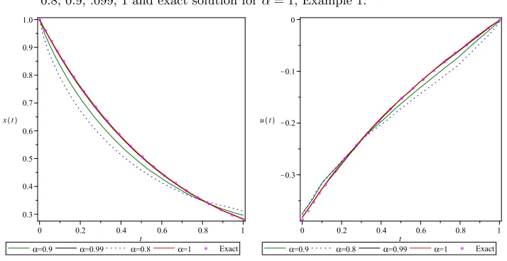
Figure 2. Approximate state and control variables forJ= 7 andα= 0.8,0.9, .099,1 and exact solution forα= 1, Example 1.

Table I. Absolute error ofx(t) with comparison to Refs, [18,22].

t Legendre basis [22] Bernollin basis [18] Biorthogonal Multiwavelet

M = 4 M = 5 M = 4 M = 5 J= 6 J= 7 J= 8

0 8.99×10−5 _6.25×10−6 _8.99×10−5 _6.25×10−6 _{0.0 0.0 0.0}

0.1 4.77×10−5 1.34×10−5 3.67×10−5 2.39×10−6 2.05×10−5 5.07×10−6 1.26×10−6 0.2 3.25×10−5 2.12×10−5 1.01×10−5 1.21×10−6 1.67×10−5 4.14×10−6 1.03×10−6 0.3 7.74×10−5 3.24×10−5 2.65×10−5 1.72×10−6 1.36×10−5 3.36×10−6 8.35×10−7 0.4 2.13×10−5 4.73×10−5 1.53×10−5 6.82×10−7 1.09×10−6 2.69×10−6 6.68×10−7 0.5 6.43×10−5 6.20×10−5 4.23×10−6 1.93×10−6 8.54×10−6 2.11×10−6 5.23×10−7 0.6 1.03×10−4 7.49×10−5 2.91×10−5 3.11×10−7 6.54×10−6 1.60×10−6 3.99×10−7 0.7 1.12×10−4 _8.88×10−5 _2.41×10−5 _1.90×10−6 _4.75×10−6 _1.17×10−6 _2.90×10−7

0.8 9.14×10−5 _1.07×10−5 _1.73×10−5 _9.17×10−7 _3.24×10−6 _7.87×10−7 _1.94×10−7

0.9 9.41×10−5 _1.31×10−5 _3.46×10−5 _2.49×10−6 _1.84×10−6 _4.44×10−7 _1.09×10−7

Table II. Estimated values forJafter thresholding, Example 1. Thresholding parameter (ε) Sparsity (Sε) J

0 0% 0.192909

J= 6 10−4 _{76.58% 0.192921}

10−3 79.20% 0.192924

10−2 _{84.46% 0.189937}

0 0% 0.192909

J= 7 10−4 85.99% 0.192912

10−3 _{87.96% 0.192999}

10−2 91.36% 0.192815

Example 2. consider the following time-varying problem [18, 22]. Find the control u(t), which minimizes the performance indexJ

MinJ(x, u) = ∫ 1

0

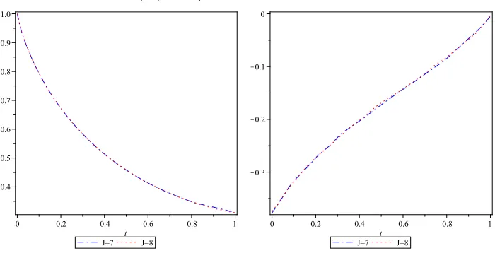
Figure 3. Comparison of state x(t) (left) and control u(t) (right) for α= 0.8 withJ= 7, 8, Example 1.

Figure 4. Plots of sparse matrices after thresholding with ε = 10−3 (left) andε= 10−2_{(right) forJ= 7, Example 1.}

subject to the following dynamics

Dαtx(t) =tx(t) +u(t), with initial condition

x(0) = 1.

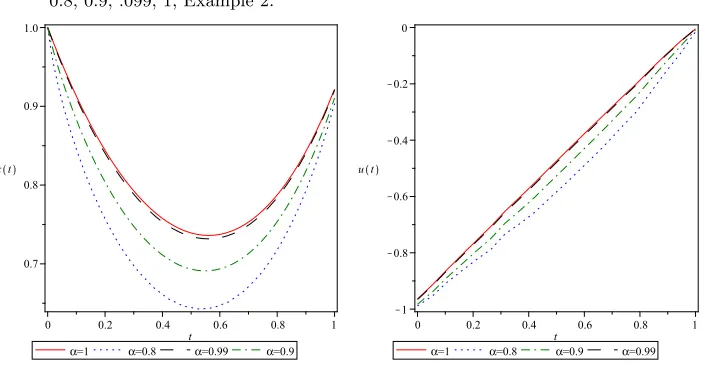
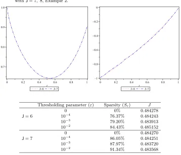
Figure 5. Approximate state and control variable for J = 7 andα = 0.8,0.9, .099,1, Example 2.

controlu(t) for different values ofα. Also we show that whenαtend to 1, the approximate solutions for both state and control variables tend to the exact solutions forα = 1. The graphs of state variablex(t) and control variableu(t) forα= 0.8 andJ= 7, 8 are plotted in Figure 6, It is obvious that with increase in the number of the biorthogonal wavelet basis, the approximate values ofx(t) andu(t) converge to the exact solutions. Table IV, reports the sparsity and minimum value ofJwhenα= 1 for different values of thresholding parameter. Also Figure 7, shows the plot of the matrix elements forJ= 7 after thresolding.

Table III. Results for Example 2

Methods J

Bernoulli basis [18]

M = 5, α= 0.8 0.466978 M = 5, α= 0.9 0.475883 M = 5, α= 0.99 0.483463

M = 5, α= 1 0.484268

Biorthogonal multiwavelets

J= 7, α= 0.8 0.466979 J= 7, α= 0.9 0.475887 J= 7, α= 0.99 0.483466

J= 7, α= 1 0.484270

J= 8, α= 0.8 0.466977 J= 8, α= 0.9 0.475883 J= 8, α= 0.99 0.483463

J= 8, α= 1 0.484268

Figure 6. Comparison of statex(t) (left) and u(t) (right) forα = 0.8 withJ= 7, 8, Example 2.

Thresholding parameter (ε) Sparsity (Sε) J

0 0% 0.484278

J= 6 10−4 _{76.37% 0.484243}

10−3 79.20% 0.483913

10−2 _{84.43% 0.485152}

0 0% 0.484270

J= 7 10−4 86.05% 0.484251

10−3 _{87.97% 0.483720}

10−2 91.34% 0.483568

6. Conclusion

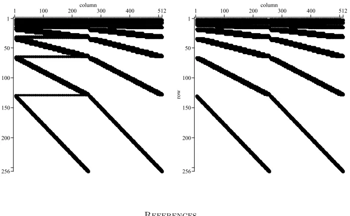
Figure 7. Plots of sparse matrices after thresholding with ε = 10−5 (left) andε= 10−4(right) forJ= 7, Example 2.

References

[1] O. M. P. Agrawal,General formulation for the numerical solution of optimal control problems, Int. J. Control.,50(1989), 627–638. DOI 10.1080/00207178908953385.

[2] O. M. P. Agrawal,A general finite element formulation for fractional variational problems, J. Math. Anal. Appl.,337(2008), 1–12. DOI 10.1016/j.jmaa.2007.03.105.

[3] O. M. P. Agrawal, Fractional variational calculus and transversality conditions, J. Phys. A:Math. Gen.,39(2006), 10375–10384. DOI 10.1088/0305-4470/39/33/008.

[4] O. M. P. Agrawal, A general formulation and solution scheme for fractional optimal control problem, Nonlinear Dynam.,38(2004), 323–337. DOI 10.1007/s11071-004-3764-6.

[5] O. M. P. Agrawal,A Hamiltonian formulation and a direct numerical scheme for fractional op-timal control problems, J. Vib. Control.,13(2007), 1269–1281. DOI 10.1177/1077546307077467. [6] O. M. P. Agrawal,A formulation and numerical scheme for fractional optimal control problems,

J. Vib. Control.,14(2008), 1291–1299. DOI 10.1177/1077546307087451.

[7] O. M. P. Agrawal, A quadratic numerical scheme for fractional optimal control problems, J. Dyn. Syst. Meas. Control.,130(1) (2008), 011010 (6pages). DOI 10.1115/1.2814055.

[8] O. M. P. Agrawal, M. Mehedi Hasan and X. W. Tangpong,A numerical scheme for a class of parametric problem of fractional variational calculus, J. Comput. Nonlinear Dyn.,7(2012), 021005–1. DOI 10.1115/1.4005464.

[9] R. Almedia and D. F. M. Torres,Calculus of variations with fractional derivatives and fractional integrals, Appl. Math. Lett.,22(2009), 1816–1820. DOI 10.1016/j.aml.2009.07.002.

[10] R. Almedia, D. F. M. Torres,Necessary and sufficient conditions for the fractional calculus of variations with Caputo derivatives, Commun. Nonlinear Sci. Numer. Simul.,16(2011), 1490– 1500. DOI 10.1016/j.cnsns.2010.07.016.

[11] D. Baleanu, O. Defterli and O. M. P. Agrawal, A central difference numerical scheme for fractional optimal control problems, J. Vib. Control., 15 (2009), 547–597. DOI 10.1177/1077546308088565.

[12] G. Beylkin, R. Coifman and V.Rokhlin,Fast wavelet transforms and numerical algorithms, I, Commun. PureAppl. Math.,44(1991), 141–183. DOI 10.1002/cpa.3160440202.

[14] P. G. Ciarlet, M. H. Schultz and R. S. Varga,Numerical methods of high-order accuracy for nonlinear boundary value problems I. One dimensional problems, Numer. Math.,9(1967) 294– 430. DOI 10.1007/BF02165273.

[15] J. C. Goswami, A. K. Chan, and C. K. Chui, On solving first-kind integral equations using wavelets on a bounded interval, IEEE Trans. Antennas propagat.,43 (1995), 614–622. DOI 10.1109/8.387178.

[16] B. Han,Approximation properties and construction of Hermite interpolants and biorthogonal multiwavelets, J. Approx. Theory.,110(2001), 18–53. DOI 10.1006/jath.2000.3545.

[17] B. Han and Q. Mo,Multiwavelet frames from refinable function vectors, Adv. Comput. Math., 18(2003), 211–245. DOI 10.1023/A:1021360312348.

[18] E. Keshavarz, Y. Ordokhani and M. Razzaghi, A numerical solution for fractional op-timal control problems via Bernoulli polynomials, J. Vib. Control., (2015), 1–15. DOI 10.1177/1077546314567181.

[19] A. A. Kilbas, H. M. Srivastava and J. J. Trujillo,Theory and Applications of Fractional Dif-ferential Equations, in:North-Holland Mathematics Studies., vol. 204, Elsevier Science B.V, Amsterdam, 2006. DOI 10.1016/S0304-0208(06)80001-0.

[20] M. Lakestani, M. Dehghan and S. Irandoust-pakchin,The construction of operational matrix of fractional derivatives using B-spline functions, Commun. Nonlinear. Sci. Numer. Simulat.,17 (2012), 1149–1162. DOI 10.1016/j.cnsns.2011.07.018.

[21] A. Lotfi, S. A. Yousefi, A numerical technique for solving a class of fractional variational problems, J. Comput. Appl. Math.,237(2013), 633–643. DOI 10.1016/j.cam.2012.08.005. [22] A. Lotfi, M. Dehghan and S. A. Yousefi,A numerical technique for solving fractional optimal

control problems, Computers and Mathematics with Applications 62(2011), 1055–1067. DOI 10.1016/j.camwa.2011.03.044.

[23] A. Lotfi, S. A. Yousefi and M. Dehghan, Numerical solution of a class of fractional op-timal control problems via the Legendre orthonormal basis combined with the operational matrix and the Gauss quadrature rule, Comput. Appl. Math., 250 (2013), 143–160. DOI 10.1016/j.cam.2013.03.003.

[24] K. B. Oldham and J. Spanier,The Fractional Calculus, NewYork: Academic Press (1974). [25] I. Podlubny,Fractional Differential Equations. (1999) NewYork: Academic Press.

[26] C. Tricaud, Y. Q. Chen, An approximation method for numerically solving fractional order optimal control problems of general form, Comput. Math. Appl.,59(2010), 1644–1655. DOI 10.1016/j.camwa.2009.08.006.