Optimization with the time-dependent Navier-Stokes equations as
constraints
Mitra Vizheh
Department of Mathematics, Shahed University, Tehran, P.O. Box: 18151-159, Iran.
E-mail:[email protected]
Sayed Hodjatollah Momeni-Masuleh∗
(shahed)Department of Mathematics, Shahed University, Tehran, P.O. Box: 18151-159, Iran.
E-mail:[email protected] Alaeddin Malek
Department of Applied Mathematics, Faculty of Mathematical Sciences, Tarbiat Modares University, Tehran, P.O. Box: 14115-134, Iran.
E-mail:[email protected]
Abstract In this paper, optimal distributed control of the time-dependent Navier-Stokes equa-tions is considered. The control problem involves the minimization of a measure of the distance between the velocity field and a given target velocity field. A mixed numerical method involving a quasi-Newton algorithm, a novel calculation of the gradients and an inhomogeneous Navier-Stokes solver, to find the optimal control of the Navier-Stokes equations is proposed. Numerical examples are given to demon-strate the efficiency of the method.
Keywords. Optimal control problems, Navier-Stokes equations,PDE-constrained optimization, quasi-Newton
algorithm, finite difference.
2010 Mathematics Subject Classification. 35Q93, 35Q30, 74S20, 90C53.
1. Introduction
Optimal control of the Navier-Stokes equations is a constrained optimization prob-lem with the Navier-Stokes equations serving as subsidiary conditions. PDE-constrained optimization problems arise in many applications and so received much progress dur-ing recent years for example Hicken and Alonso [14] described an algorithm for PDE-constrained optimization that controls numerical errors. Akbarian and Keyanpour [1] proposed a new numerical method for solving a class of fractional order optimal con-trol problems. The fractional optimal concon-trol theory is a new topic in Mathematics. Kar [17] discussed an optimal control problem in population dynamics.
Received: 6 June 2015 ; Accepted: 3 February 2016. ∗Corresponding Author.
In general, optimal control problems are classified into distributed and boundary con-trol problems. In the case of additional constraints, optimal concon-trol problems rather than the Navier-Stokes equations are divided into four groups: (i) State-constrained [8], (ii) Control-constrained [25], (iii) mixed state-control constrained [9] and (iv) op-timal control of the Navier-Stokes equations without inequality constraints [16], [13]. Hinze and Kunisch [16] have used second order methods for optimal control of the time-dependent Navier-Stokes equations for the first time. Hinze [15] has delivered a good literature review up to 2002 in his research report.
Li et al. [19] have presented a general method based on adjoint formulation for the optimal control of distributed parameter systems and applied it to the problem of controlling vortex shedding behind a cylinder governed by the unsteady two dimen-sional Navier-Stokes equations with time-dependent boundary conditions. They used a quasi-Newton Daviden-Fletcher-Powell (DFP) method for the minimization of the cost function. Chaabane et al. [4] have considered a non-convex cost function of the velocity gradient tensor and provide the optimality systems based on a lagrangian formulation and adjoint equations. Optimal boundary control problems for the three dimensional evolutionary Navier-Stokes equations in the exterior of a bounded do-main are investigated by Fursikov et al. [10], theoretically. In their work the drag functional is minimized as a control objective. The problem of an appropriate choice of a cost functional for vortex reduction for unsteady flows is considered by Kunisch and Vexler [18]. Brizitskii [3] has studied optimal control problems for the station-ary Navier-Stokes equations with mixed boundstation-ary conditions on velocity and derived some theorems on the uniqueness and stability of solutions for the particular func-tional that depend on the total pressure. Bili´c in [2] has derived some theoretical results for the optimal control of a coefficient in modification of the Navier-Stokes equations. She considered the coefficient of the kinematic viscosity to be a positive function of the velocity gradient. Recently, the existence of optimal solution and the maximum principle for optimal control problem of Navier-Stokes equations with state constraint of point wise type in three dimensions are studied by Liu [20].
The paper is organized as follows. In Section 2, we will briefly review some theory in optimal control of the Navier-Stokes equations. Section 3 gives details of the op-timization method applied for the optimal control problem and deals with numerical solution of the inhomogeneous Navier-Stokes equations. Numerical results are given in Section 4.
2. Optimal control of Navier-Stokes equations
Let Ω⊂R2be a bounded domain with∂Ω∈ C2. Solenoidal spaces are introduced as follows
H :={v∈C∞
0 2: divv= 0}
−|·|L2(Ω)2,
V :={v∈C0∞ 2
: divv= 0}−|·|H1(Ω)2,
where the superscripts denote closures in the respective norms. Optimal distributed control of the Navier-Stokes equations is given by [15]
min (u,f)∈W×U
J(u,f),
s.t.:
∂u
∂t + (u· ∇)u− 1
Re∆u+∇p=f, inΩ×(0, T),
∇ ·u= 0, inΩ×(0, T),
u(t,·) = 0, on(∂Ω)×(0, T),
u(0,·) =u0, inΩ, (2.1)
whereu: [0, T]×Ω→R2 is the velocity field,p: [0, T]×Ω→Ris the pressure field, f : [0, T]×Ω→ R2 is the control function, T is the final time, Re is the Reynolds number, u0 is a given initial velocity field and U is the Hilbert space of controls. Further we defineW to be
W ={v∈L2(V) :vt∈L2(V∗)},
with the associated norm
|v|W =|v|L2(V)+|vt|L2(V∗),
whereV∗ is the dual space ofV.
In this paper, we consider the tracking type objective functional
J(u,f) = 1 2
Z T
0
Z
Ω
|u−z|2dxdydt+α 2|f|
2
Herez is a given velocity of a target flow andαis a penalty parameter. It is assumed thatJ is bounded from below, weakly lower semi-continuous, twice Fr´echet differen-tiable with locally Lipschitzean second derivative and radially unbounded inf. Thanks to Theorem 2.1 in Ref. [15] for every f ∈U, there exists a unique element u = u(f) satisfying the Navier-Stokes equations, therefore problem (2.1) can be equivalently written as
min f∈U
ˆ
J(f) =J(u(f),f).
Theorem 2.1.Under above assumptions, problem(2.1)admits a solution(u∗(f∗),f∗)∈
W×U.
Proof. See [15].
2.1. Lid driven cavity control. Let us consider the lid driven cavity control of the Navier-Stokes equations in two dimensions as follows
(p) : minJ(u, v, f1, f2) =1 2
Z 1
0
Z 1
0
Z 1
0
[(u−z1)2+ (v−z2)2]dxdydt
+α 2
Z 1
0
Z 1
0
Z 1
0
(f12+f22)dxdydt,
s.t.:
ut+px+u·ux+v·uy−
1
Re(uxx+uyy) =f1, inΩ×(0, T),
vt+py+u·vx+v·vy−
1
Re(vxx+vyy) =f2, inΩ×(0, T), ux+vy= 0, inΩ,
u= 1, v= 0, Γ1: 0≤x≤1, y= 1,
u= 0, v= 0, Γ2: 0≤x≤1, y= 0,
u= 0, v= 0, Γ3:x= 0,0≤y≤1,
u= 0, v= 0, Γ4:x= 1,0≤y≤1,
u(0,·) = 0, inΩ,
v(0,·) = 0, inΩ, (2.2)
3. Numerical solution for the optimal control problem
In this section we present a typical optimization algorithm as follows [11].
Algorithm.
Start with an initial guessf0= (f0
1, f20) for the control vector. Then forn= 0,1,2, ...
(1) Solve the Navier-Stokes equations to obtain the corresponding state un= (un, vn),
(2) Compute ddfJˆ|fn,
(3) Use the results of steps (1) and (2) to compute an optimal directionδf, (4) setfn+1 =fn+δf.
For the step (1) and step (3) we use a Navier-Stokes solver and the quasi-Newton Broyden-Fletcher-Goldfarb-Shanno (BFGS) algorithm [21], respectively. For the step (2) we use the following method. By the chain rule we have
ˆ J′ =
∂J ∂f1 ∂J ∂f2 = ∂J1 ∂u · ∂u ∂f1 +
∂J2
∂f1
∂J1
∂v · ∂v ∂f2 +
∂J2 ∂f2 , where
J1=1 2 Z 1 0 Z 1 0 Z 1 0
[(u−z1)2+ (v−z2)2]dxdydt,
J2=α 2 Z 1 0 Z 1 0 Z 1 0
(f12+f22)dxdydt,
The terms ∂J2
∂f1,
∂J1
∂v, ∂J1
∂u and ∂J2
∂f2 are as follows [15]
∂J1
∂u =u−z1, ∂J1
∂v =v−z2, ∂J2
∂f1 =αf1, ∂J2 ∂f2 =αf2.
For the terms ∂f∂u1 and ∂f∂v2, we use the finite difference approximation [11]
∂u ∂f1|f
n
1 = u(fn
1)−u(f1) fn
1 −f1 ,
∂v ∂f2|f2n=
v(fn
2)−v(f2) fn
2 −f2 ,
wheref1 andf2 are some values close tofn
1 andf2n, respectively.
mitnavierstokes1806.m, have been extended to inhomogeneous Navier-Stokes equa-tions using Strang’s general approach [24]. Now, we present a brief summary of the numerical solution approach. While (u, v) and p are the solutions to the Navier-Stokes equations, we denote the numerical approximations by capital letters. Assume we have the velocity field Un and Vn at the nth time step and condition (2.2) is
satisfied. We find the solution at the (n+ 1)th time step by the following three step
approach:
• Explicit treatment of the nonlinear terms U∗−Un
∆t =−((U
n)2)
x−(UnVn)y+f1n,
V∗−Vn
∆t =−(U
nVn)
x−((Vn)2)y+f2n,
• Implicit treatment of the viscosity terms U∗∗−U∗
∆t =
1 Re(U
∗∗
xx+U
∗∗
yy),
V∗∗−V∗
∆t =
1 Re(V
∗∗
xx +Vyy∗∗),
• Pressure correction
We correct the intermediate velocity field (U∗∗, V∗∗) by the gradient of a pressurePn+1 to enforce incompressibility.
Un+1−U∗∗
∆t =−(P
n+1)
x,
Vn+1−V∗∗
∆t =−(P
n+1)
y,
in vector notation the correction equations read as 1
∆tU
n+1− 1 ∆tU
n =−∇Pn+1.
Applying the divergence to both sides of the above equation yields the fol-lowing linear system of equations.
−∆Pn+1=− 1
∆t∇ ·U
n.
4. Numerical results
set to ∆t= 0.01 and ∆x= ∆y= 1/76, respectively.
Example 1. In this example we consider the Stokes flow as the target flow. To
do this, the Navier-Stokes equations with a Reynolds number that was very smaller than one is solved as the target flow. A Navier-Stokes flow with Reynolds number equal to 10 matches the target flow in the beginning time steps.
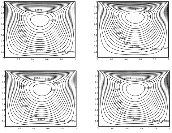
The target flow and the controlled flow at t = 0, t = 0.3 and t = 1 are shown in Figure1. The figure shows that a good match is achieved at the time t=0.3.
Furthermore, the infinity norm of (U−z) between the controlled flow and the target flow and the infinity norm off of the optimal control versus time is shown in Figure2. As one can see the errorkU−zk goes to zero and the norm of the control becomes relatively large at the beginning in order to steer the controlled flow to the target flow and then after a good match is achieved, its norm remains relatively constant. Table1
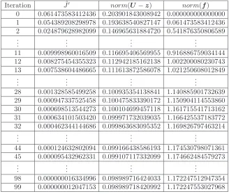
demonstrates the infinity norm of approximate gradient, the difference between the controlled flow and the target flow and the control variable, respectively.
Example 2. Here, we have solved the Navier-Stokes equations with a Reynolds
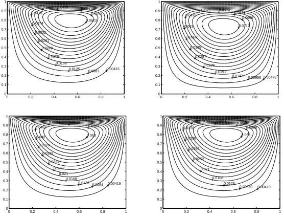
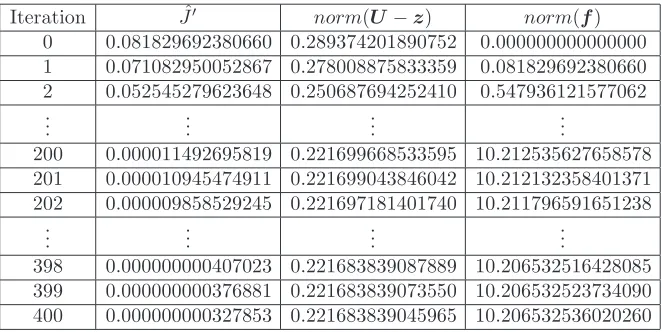
number equal to 100 and obtained the velocity of the target flow. The target flow is a Navier-Stokes flow with Reynolds number equal to 100. In this case, a flow with Reynolds number equal 20 is made close enough to the target flow. Similar results are obtained that is shown in figures3and4 and Table2.
These examples confirm that the proposed method works well in making close enough a Navier-Stokes flow with low Reynolds number to a Navier-Stokes flow with higher Reynolds number and vice versa.
5. Conclusion
In this article, we have combined several mathematical methods including a quasi-Newton algorithm, a new calculation of the gradients and a Navier-Stokes solver, to solve the optimal control of the time-dependent Navier-Stokes equations. We have extended a homogeneous Navier-Stokes solver to an inhomogeneous one and used it for the optimization problem.
References
[1] T. Akbarian and M. Keyanpour,A new approach to the numerical solution of fractional order optimal control problems, Applications And Applied Mathematics, 8 (2013), 523-534.
[2] N. Bili´c,Optimal control of a cofficient in modification Navier-Stokes equations, Math. Slovaca
60, 1 (2010), 83-96.
[3] R. V. Brizitskii,Study of a class of control problems for the stationary Navier-Stokes equations with mixed boundary conditions, Institute of Applied Mathematics, ul. Radio 7, Vladivostok, 690041 Russia, 2008.
[4] S. Chaabane, J. Ferchichi, K. Kunisch,Optimal distributed control of vortices in Navier-Stokes flow, C. R. Acad. Sci. Paris, Ser. I 341, 2005.
[5] A.J. Chorin, J.E. Marsden, A Mathematical Introduction to Fluid Mechanics, Third Edition, Springer, 2000.
[6] K. Chrysafinos,Analysis and finite element approximation for distributed optimal control prob-lems for implicit parabolic equations, Journal of Computational and Applied Mathematics, 231 (2009), 327-348.
[7] J. C. De Los Reyes,Regularized state-constrained boundary control of the Navier-Stokes equa-tions, J. Math. Anal. Appl. 357, 1 (2009), 257-279.
[8] J. C. de los Reyes and K. Kunisch, A semi-smooth newton method for regularized state-constrained optimal control of the Navier-Stokes equations, Computing 78 (2006), 287-309. [9] J. C. de los Reyes and F. Tr¨oltzsch,Optimal control of the stationary Navier-Stokes equations
with mixed control-state constraints, SIAM Journal on Control and Optimization, 46(2) (2007), 604-629.
[10] A. V. Fursikov, M. D. Gunzburger and L. S. Hou,Optimal boundary control for the evolutionary Navier-Stokes system: The three dimensional case, SIAM J. Control Optim. 43 (2005), 2191-2232.
[11] M. Gunzburger,Adjoint equation-based methods for control problems inincompressible, viscous flows, Flow, Turbulence and Combustion 65 (2000), 249-272.
[12] H. Heidari and A. Malek,Null boundary controllability for hyperdiffusion equation, Int. J. App. Math. 22,(4) (2009), 615-626.
[13] M. Heinkenschloss, Formulation and analysis of a sequential quadratic programming method for the optimal dirichlet boundary control of Navier-Stokes flow, in Optimal Control: Theory,
Algorithms and Applications, Kluwer Academic Publishers B. V. ,1998.
[14] J.E. Hicken and J.J. Alonso (2014),PDE-constrained optimization with error estimation and control, Journal of Computational Physics, 263 (2014), 136-150.
[15] M. Hinze,Optimal and instantanous control of the instationary Navier-Stokes equations, Insti-tute f¨ur Numerische Mathematik, Technische Universit¨at Dresden, 2002.
[16] M. Hinze and K. Kunisch,Second order methods for optimal control of time-dependent fluid flow, Karl-Franzens Universit¨at Graz, Institut f¨ur Mathematik, Spezialforschungsbereich F003, Bereich 165, 1999.
[18] K. Kunisch and B. Vexler,Optimal vortex reduction for instationary flows based on translation invariant cost functional, SIAM J. Control Optim,vol. 46, Issue 4(2007), 1368-1397.
[19] Z. Li, I. M. Navon, M. Y. Hussaini and F. X. L. Dimet,Optimal control of cylinder wakes via suction and blowing, Computers and Fluids 32(2003), 149-171.
[20] H. Liu,Optimal control problems with state constraint governed by Navier-Stokes equations, Nonlinear Analysis 73(2010), 3924-3939.
[21] J. Nocedal and S. J. Wright,Numerical Optimization, Springer, 1999.
[22] R. W. H. Sargent,Optimal control, Journal of Computational and Applied Mathematics (2000), 361-371.
[23] B. Seibold,A compact and fast matlab code solving the incompressible Navier-Stokes equations on rectangular domains, Massachusetts Institute of Technology, 2008.
[24] G. Strang,Computational Science and Engineering, First Edition, Wellesley Cambridge Press, 2007.
[25] M. Ulbrich,Constrained optimal control of Navier-Stokes flow by semismooth newton methods, Systems and control letters 48(2003), 297-311.
Table 1. Performance of the BFGS algorithm for Example 1.
Iteration Jˆ′ norm(U −z) norm(f)
0 0.061473583412436 0.203901843008942 0.000000000000000 1 0.054389208298978 0.193638540827147 0.061473583412436 2 0.024879628982099 0.146965631884720 0.541876350806589
..
. ... ... ...
11 0.009998960016509 0.116695406569955 0.916886759034144 12 0.008275454355323 0.112942185162138 1.002200080230743 13 0.007538604486665 0.111613872586078 1.021250608012849
..
. ... ... ...
28 0.001328585499258 0.100935354138841 1.140885901732639 29 0.000947337525458 0.100475833390172 1.150904114553860 30 0.000698513544273 0.100104699457118 1.161715541713162 31 0.000634101503420 0.099971732039035 1.166425537183772 32 0.000462344144686 0.099863683095352 1.169826797463214
..
. ... ... ...
44 0.000124632802094 0.099166438586193 1.174530798071361 45 0.000095432962331 0.099107117332099 1.174662484579273
..
. ... ... ...
Figure 1. Streamlines of target flow (top left), streamlines of con-trolled flow at t=0 (top right), streamlines of concon-trolled flow at t=0.3 (bottom left) and streamlines of controlled flow at t=1 (bottom right) for Example 1.
0.00441 0.00883 0.0132 0.0177 0.0221 0.0265 0.0309 0.0353 0.0397 0.0441 0.0485 0.053 0.0574 0.0618 0.0662
0 0.2 0.4 0.6 0.8 1 0 0.1 0.2 0.3 0.4 0.5 0.6 0.7 0.8 0.9 1 0.0047 0.00941 0.0141 0.0188 0.0235 0.0282 0.0329 0.0376 0.0423 0.047
0.0517 0.0564 0.0611 0.0658
0.0705
0 0.2 0.4 0.6 0.8 1 0 0.1 0.2 0.3 0.4 0.5 0.6 0.7 0.8 0.9 1 0.00433 0.00867 0.013 0.0173 0.0217 0.026 0.0303 0.0347 0.039 0.0433
0.0477 0.052 0.0564 0.0607
0.065
0 0.2 0.4 0.6 0.8 1 0 0.1 0.2 0.3 0.4 0.5 0.6 0.7 0.8 0.9 1 0.00433 0.00866 0.013 0.0173 0.0216 0.026 0.0303 0.0346 0.039 0.0433 0.0476 0.0519 0.0563 0.0606 0.0649
0 0.2 0.4 0.6 0.8 1 0 0.1 0.2 0.3 0.4 0.5 0.6 0.7 0.8 0.9 1
Figure 2. The normkfkof the optimal control (left) and the norm
kU−zk between the controlled flow and the target flow (right) vs. time for Example 1.
0 0.2 0.4 0.6 0.8 1 0 0.2 0.4 0.6 0.8 1 1.2 1.4 t ||f||
Figure 3. Streamlines of target flow (top left), streamlines of con-trolled flow at t=0 (top right), streamlines of concon-trolled flow at t=1 (bottom left) and streamlines of controlled flow at t=4 (bottom right) for Example 2.
0.00415 0.0083 0.0125 0.0166 0.0208 0.0249 0.0291 0.0332 0.0374 0.0415
0.0457 0.0499 0.054 0.0582 0.0623
0 0.2 0.4 0.6 0.8 1 0 0.1 0.2 0.3 0.4 0.5 0.6 0.7 0.8 0.9 1 0.00478 0.00956 0.0143 0.0191 0.0239 0.0287 0.0335 0.0382 0.043 0.0478 0.0526 0.0574 0.0621 0.0669 0.0717
0 0.2 0.4 0.6 0.8 1 0 0.1 0.2 0.3 0.4 0.5 0.6 0.7 0.8 0.9 1 0.00419 0.0084 0.0126 0.0168 0.021 0.0252 0.0294 0.0336 0.0378 0.042 0.0462 0.0504 0.0546 0.0588 0.063
0 0.2 0.4 0.6 0.8 1 0 0.1 0.2 0.3 0.4 0.5 0.6 0.7 0.8 0.9 1 0.00419 0.00839 0.0126 0.0168 0.021 0.0252 0.0294 0.0336 0.0378
0.042 0.0462 0.0504 0.0546 0.0588
0.063
0 0.2 0.4 0.6 0.8 1 0 0.1 0.2 0.3 0.4 0.5 0.6 0.7 0.8 0.9 1
Figure 4. The normkfkof the optimal control (left) and the norm
kU−zk between the controlled flow and the target flow (right) vs. iteration for Example 2.
0 20 40 60 80 100
0 1 2 3 4 5 6 7 8 9 10
0 20 40 60 80 100
Table 2. Performance of the BFGS algorithm for Example 2.
Iteration Jˆ′ norm(U−z) norm(f)
0 0.081829692380660 0.289374201890752 0.000000000000000 1 0.071082950052867 0.278008875833359 0.081829692380660 2 0.052545279623648 0.250687694252410 0.547936121577062 ..
. ... ... ...
200 0.000011492695819 0.221699668533595 10.212535627658578 201 0.000010945474911 0.221699043846042 10.212132358401371 202 0.000009858529245 0.221697181401740 10.211796591651238
..
. ... ... ...