Solution of Troesch
,s problem through double exponential
Sinc-Galerkin method
Mohammad Nabati∗
Department of Basic Sciences, Abadan Faculty of Petroleum Engineering, Petroleum University of Technology, Abadan, Iran.
E-mail: [email protected]
Mahdi Jalalvand
Department of Mathematics, Faculty of Mathematical Sciences and Computer, Shahid Chamran University of Ahvaz, Ahvaz, Iran.
E-mail: [email protected]
Abstract Sinc-Galerkin method based upon double exponential transformation for solving Troesch,s problem is given in this study. Properties of the Sinc-Galerkin approach
are utilized to reduce the solution of nonlinear two-point boundary value problem to same nonlinear algebraic equations, also, the matrix form of the nonlinear algebraic equations is obtained.The error bound of the method is found. Moreover, in order to illustrate the accuracy of presented method, the obtained results compare with numerical results in the open literature. The demonstrated results confirm that proposed method is considerably efficient and accurate.
Keywords. Sinc Function, Galerkin method, Double exponential transformation, Nonlinear Troesch,s problem, BVP.
2010 Mathematics Subject Classification. 65L10, 65L60, 65H10, 41A30.
1. Introduction
Sinc approximation methods have been proposed and studied by F. Stenger since 1974 [18]. These methods have been recognized as powerful tools for solving a wide range of linear and nonlinear problems arising from scientific and engineering appli-cations. It is well known that the approximation by Sinc approaches has the order of accuracyO
(
exp(−k√n) )
where C is a positive constant and n is the number of node or bases functions used in the method [12, 19].
In 2002, Sugihara composed Sinc function by double exponential transformation, discovered by Mori [22], and found that the error of new method isO
(
exp(−k′n/logn) )
with some positivek′ [20,21].
In the current study, application of Sinc-Galerkin method based on double expo-nential transformation (DE) to solve Troesch,s problem is developed.
Received: 4 January 2017 ; Accepted: 22 April 2017.
∗Corresponding author.
Troesch,s problem is a special nonlinear two point boundary value problem, defined
as
y′′(x) =msinh(m y(x)), 0< x <1
y(0) = 0, y(1) = 1,
(1.1)
where ′m′ is a positive constant. This problem arises in an investigation of the confinement of a plasma column by radiation pressure [25] as well as in the theory of gas porous electrodes [7,13].
The closed form solution to this problem in terms of the Jacobian elliptic function has been given [5] as
y(x) = 2
msinh
−1{y′(0)
2 Sc (
m x|1−1 4y
′(0)2)}, (1.2)
wherey′(0) (the derivation ofyatx= 0) is given by expressiony′(0) = 2√1−t, with
tbeing the solution of the transcendental equation sinh(m2)
√
1−t =Sc(m|t), (1.3)
where the Jacobian elliptic function Sc(m|t) is defined by Sc(m|t) = tanϕ, where
ϕ, mare related through the integral below
m= ∫ ϕ
0
1 √
1−t−sin2θ
dθ. (1.4)
It has been shown thaty′(x) has a singularity located approximately at [15, 24]
χs= 1
mln
( 8
y′(0) )
, (1.5)
which implies that the singularity lies the integration range ofy′(0)>8e−η.
Many of researches have been conducted to study and solved this problem by ap-proximation methods. Chang [1] applied shooting method, Xinlong et al [5] used an modified homotopy perturbation method, Zarebnia et al. [26] developed Sinc-Galerkin method based on single exponential (SE) transformation. They found that the rate of convergence by using Sinc-Galerkin method based on SE transformation is
O
(
exp(−k√n) )
. EL-Gamel [6] applied Sinc-collocation method based on SE trans-formation. Deeba et al. [3] proposed decomposition approximation method. Saadat-mandi et al. [16] applied Christov rational functions and collocation points, Khuri et al. [5] developed B-Spline method, Scott [17] used an invariant imbedding method.
The rest of the paper is organized into five sections. A brief introduction to the Sinc function, definitions, theorems and notations is presented in Section 2. In Section 3, Sinc-Galerkin method based on DE transformation to solve Troesch,s problem was
2. SINC FUNCTION PROPERTIES
In this section, some properties of the Sinc function, quadrature as well as its notations to be reviewed.
The Sinc function is defined on the whole real line,−∞< x <∞, by
Sinc(x) =
{ sin(πx)
πx , x̸= 0,
1, x= 0.
For anyh >0, the translated Sinc function with evenly spaced nodes are given as
S(j, h)(x) = Sinc
(x−jh
h
)
, j= 0,±1,±2, .... (2.1)
TheS(j, h) is called thejth Sinc function with step sizehat x.
Lemma 2.1. [12]Let S(k, h)(x)is thekth Sinc function with steph, so
δjk(0)=S(j, h)(kh) = {
1, j=k,
0, j̸=k,
δjk(1)=hd
dz[S(j, h)(z)](kh) =
{
0, j=k, (−1)k−j
k−j , j̸=k,
δjk(2)=h2 d 2
dz2[S(j, h)(z)](kh) =
{
−π2
3 , j=k,
−2(−1)k−j
(k−j)2 , j̸=k.
For the assembly of the discrete system, it is convenient to define the following matrices
I(l)= [δjk(l)] l= 0,1,2, (2.2)
whereδjk(l)denotes the (j, k)th element of the matrixI(l). The matrixI(0)is them×m
identity matrix. The matrixI(1) is the skew symmetric Toeplitz matrix andI(2) is
the symmetric Toeplitz matrix.
The following notation will be necessary for writing down the system. LetD(g) be them×mdiagonal matrix
D
(
g(x) )
=
g(−N h) 0 0 . . . 0
0 g((−N+ 1)h) 0 . . . 0
..
. . .. ...
0 . . . 0 g((N h))
.
If the functionf is defied on the real line, then forh >0 the series
C(f, h)(x) =
∞
∑
j=−∞
f(jh)Sinc
(x−jh
h
)
is called the Whittaker cardinal expansion off where this series converges [19]. These properties are derived in the infinite stripDd of the complex plane, where for d >0
Dd =
{
w=ξ+iη:|η|< d < π
2 }
.
To state the decay property of functions precisely, we introduce the following func-tion space. LetH1(D
d) be a function space defined as
H1(Dd) ={f :Dd→C|f is analytic on Dd and N1(f, Dd)<∞},
where
N1(f, Dd)≡lim
ε→0
∫
∂Dd(ε)
|f(t)| |dt|,
Dd(ε) ={ t∈C| |Re t| ≤1/ε, |Im t| ≤d(1−ε)}.
Theorem 2.2. [23]Assume that a function f satisfies
1)f ∈H1(Dd),
2)∀x∈R:|f(x)|≤Aexp(−B exp(γ |x|)), for positive constantsA, B,γ anddwhere γd≤ π
2. Then there exists a constant C independent ofN, such that
sup
−∞<x<∞
f(x)−
N
∑
k=−N
f(kh)S(k, h)(x)≤Cexp (
− πdγN
log(πdγN/B) )
,
where
h= log(πdγN/B)
γN .
Theorem 2.3. [20]Ford >0, letf be a holomorphic function onDd such that
N(f, d)≡ lim
ε→0+
∫ ∞
−∞
(|f(x+i(d−ε))|+|f(x−i(d−ε))|)dx <∞, (2.3)
lim
ε→0+
∫ −(d−ε)
(d−ε)
|f(x+iy)|dy= 0, (2.4)
for arbitraryεwith 0< ε <1, and
∀xϵR: |f(x)|≤Aexp(−B exp(γ |x|)), (2.5)
for constants A, B > 0 and γ > 0 with γd ≤ π2. Then there exists a constant C independent ofN, such that
∫ ∞
−∞
f(x)dx−h N
∑
k=−N
f(kh)≤Cexp (
− 2πdγN
log(2πdγN/B) )
, (2.6)
where
h= log(2πdγN/B)
3. DE-Sinc-Galerkin Method for Troesch,s Problem Consider Troesch,s problem as
L(y(x))≡y′′(x)−m sinh(m y(x)) = 0, 0< x <1,
y(0) = 0, y(1) = 1.
(3.1)
Before illustrating Sinc-Galerkin method based on DE transformation, we need to convert the nonhomogeneous boundary conditions to homogeneous ones. For this purpose the change of variableu(x) =y(x)−xwas considered. So by applying this change of variable the above problem is converted to
L(u(x))≡u′′(x)−m sinh(m u(x) +m x) = 0, 0< x <1,
u(0) = 0, u(1) = 0.
(3.2)
Since the suitable domain for Sinc function is (−∞,∞), so for problems with another domain, there are two points of view. The first is to change of variables in the problem so that, in new variables, the problem has a domain corresponding to (−∞,∞). The second procedure is to move the numerical process and study it on original domain of problem. The former approach is chosen here. For our problem with domain (0,1), the appropriate transformation is following conformal map
x=ψ(t) =1 2tanh
(π 2sinh(t)
) +1
2, (3.3)
t=ϕ(x) =ψ−1(x) = log [1
πlog( x
1−x) +
√ 1 +
(1
πlog( x
1−x)
)2]
, (3.4)
which is called double exponential (DE) transformation and Sinc-Galerkin method based on this transformation is called DE-Sinc-Galerkin method. This DE transfor-mation [22,23] maps Ronto (0,1) and maps Dd onto the domain
ψ(Dd) = {
zϵC:arg (1
πlog( z
1−z) +
√ 1 +
(1
πlog( z
1−z)
)2)
< d
}
.
By applying ψ to problem (3.2), this problem is transformed to new one on (−∞,∞) as follows
L(u(ψ(t)))≡ d2
dx2u(ψ(t))−m sinh(m u(ψ(t)) +m ψ(t)) = 0,
limt→±∞u(ψ(t)) = 0.
(3.5)
Setv(t) =u(ψ(t)), so by chain rule of differentiation we obtain
d
dxu(ψ(t)) =
1
ψ′(t)v
′(t), (3.6)
d2
dx2(u(ψ(t))) =
( 1
ψ′(t) )2
v′′(t)− ψ
′′(t)
(ψ′(t))3v
By using the formulas (3.6) and (3.7) in eq (3.5) and multiply by (
ψ′(t) )
we have
L(v(t))≡ψ′1(t)v′′(t) +
(
− ψ′′(t) (ψ′(t))2
)
v′(t)−m
(
ψ′(t) )
sinh (
mv(t) +mψ(t) )
= 0,
limt→±∞v(t) = 0.
(3.8)
To approximate the solution of problem (3.8) the Sinc approximation by the fol-lowing formula was considered
vr(t) = N
∑
j=−N
cjSj(t), r= 2N+ 1, (3.9)
where the bases Sinc functionsSj(t) =S(j, h)(t) are defined in (2.1) and the unknown coefficients{cj}N
k=−N need to be determined. Notice that thevrsatisfies the boundary
conditions because of limt→±∞Sj(t) = 0.
Our purpose is to apply the Sinc-Galerkin method based on DE transformation on the problem (3.8). At first, the following form of inner product for arbitrary function
f andgwas considered as
≺f, g≻= ∫ +∞
−∞
f(t)g(t)w(t)dt, (3.10)
where w(t) is a weight function. The weight function in the Sinc-Galerkin inner product may be chosen based on a variety of reasons. For instance, Lund [12] used a kind of w for symmetrization of system in a self-adjoint linear problems, but the selection that we make here is due to the requirement of vanishing the boundary terms when using the integration by part in inner product. In this case, we usew(t) =ψ′(t). For more information about different choices of the weight function see [12,14,18].
The coefficients{cj}N
j=−N are determined by orthogonalizing the residualLvwith
respect to the functions {
Sk(x)
}N
k=−N
, in other words
≺Lv, Sk ≻= 0, k =−N,−N+ 1, ..., N. (3.11)
So we have
≺ 1
ψ′(t)v
′′(t), Sk(t)≻ − ≺ ψ′′(t)
(ψ′(t))2v
′(t), Sk(t)≻
− ≺ψ′(t)msinh(mv(t) +mψ(t), Sk(t)≻= 0,
By considering the inner product in (3.10), the above inner products are calculated as follow
≺ψ′(t)msinh(mv(t)+mψ(t)), Sk(t)≻=
∫ +∞
−∞
(
ψ′(t) )2
msinh(mv(t) +mψ(t))Sk(t)dt. (3.13)
By applied quadrature formula in Theorem 2.3, we obtain
∫ +∞
−∞
(
ψ′(t) )2
msinh(mv(t) +mψ(t))Sk(t)dt−
h
((
ψ′(kh) )2
msinh(mck+mψ(kh)))≤C0exp
(
− k′N
log(k′N/B) )
, (3.14)
wherehis defined in (2.7) andk′ = 2πdγ. Another inner product is
≺ ψ′′(t) (ψ′(t))2v
′(t), Sk(t)≻=∫ +∞ −∞
ψ′(t) ψ
′′(t)
(ψ′(t))2v
′(t)Sk(t)dt (3.15)
=v(t)ψ
′′(t)
(ψ′(t)Sk(t) +∞
−∞−
∫ +∞
−∞ v(t)
[( ψ′′(t)
(ψ′(t)) )′
Sk(t) + ψ
′′(t)
(ψ′(t))S
′ k(t)
]
dt,
but limt→±∞Sk(t) = 0, limt→±∞v(t) = 0, limt→±∞ψ
′′
ψ′(t) = 0. So the integration of
(3.15) is equal to
− ∫ +∞
−∞ v(t)
[( ψ′′(t)
(ψ′(t)) )′
Sk(t) + ψ
′′(t)
(ψ′(t))S
′ k(t)
]
dt. (3.16)
Based on quadrature formulas in Theorem 2.3 we have
∫ +∞
−∞ v(t)
[( ψ′′(t)
(ψ′(t)) )′
Sk(t) + ψ
′′(t)
(ψ′(t))S
′ k(t)
]
dt−
h N
∑
j=−N v(jh)
[(ψ′′(jh)
(ψ′(jh)) )′
Sk(jh) + ψ
′′(jh)
(ψ′(jh))S
′
k(jh)] (3.17)
≤C1exp
(
− k′N
log(k′N/B) )
.
So
≺ 1
ψ′(t)v
′′(t), Sk(t)≻=∫ +∞ −∞
v′′(t)Sk(t)dt. (3.18)
By twice integration by part we can evaluate above integration as follows
≺ 1
ψ′(t)v
′′(t), Sk(t)≻=v′(t)Sk(t)−v(t)S′ k(t) +
∫ +∞
−∞
According to the boundary conditions and limt→±∞Sk(t) = 0, and based on
quadra-ture formulas in Theorem 2.3 we get
∫ +∞
−∞
v(t)Sk′′(t)dt−h N
∑
j=−N
v(jh)Sk′′(jh)≤C2exp
(
− k′N
log(k′N/B) )
.
(3.20) To find the discrete system for equation (3.11) considering (3.12), (3.14), (3.17), (3.20) we have
≺Lv, Sk ≻ −h N
∑
j=−N v(jh)
{
S′′k(jh) +
(ψ′′(jh)
(ψ′(jh)) )
Sk′(jh)+
(ψ′′(jh)
(ψ′(jh)) )′
Sk(jh)
} −h
(
ψ′(kh) )2
msinh(mv(kh) +mψ(kh))
≤≺ 1
ψ′(t)v
′′(t), Sk(t)≻ −h N
∑
j=−N
v(jh)Sk′′(jh)+
≺ ψ′′(t)
(ψ′(t))2v′(t), Sk(t)≻ −h N
∑
j=−N v(jh)
[( ψ′′(jh)
(ψ′(jh)) )′
Sk(jh)+
ψ′′(jh) (ψ′(jh))S
′
k(jh)]+≺ψ′(t)msinh(mv(t) +mψ(t)), Sk(t)≻ −
h
((
ψ′(kh) )2
msinh(mv(kh) +mψ(kh)))
≤(C0+C1+C2
) exp
( −k′N
log(k′N/B) )
. (3.21)
Deleting the error term of orderO
( exp
(
− k′N log(k′N/B)
))
, replacingv(jh) bycj, di-viding byh, and by considering the definition ofδkj(l)we have the following nonlinear algebraic system
N
∑
j=−N cj
{1
h2δ (2) kj+
1
h
( ψ′′(jh)
(ψ′(jh)) )
δ(1)kj +
( ψ′′(jh)
(ψ′(jh)) )′
δkj(0)
} − (
ψ′(kh) )2
msinh(mck+mψ(kh)) = 0,
k=−N,−N+ 1, ..., N−1, N. (3.22) For convenience, by recalling the notations in Section 2, we can writing down the nonlinear algebraic system of (3.22) as matrix-vector form. LetCbe the r-vector with
jthcomponent given byc
j, and sinh(m C+m ψ) be the r-vector withjthcomponent
given by sinh(m cj+m ψ(jh)). Thus, the nonlinear algebraic system is rewriting as
follow
AC+Bsinh (
m C+m ψ
)
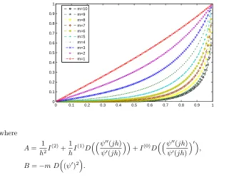
Figure 1. Approximation solution form= 1,2, ...,10 for Troesch,s Problem
in this study.
0 0.1 0.2 0.3 0.4 0.5 0.6 0.7 0.8 0.9 1
0 0.1 0.2 0.3 0.4 0.5 0.6 0.7 0.8 0.9 1
m=10 m=9 m=8 m=7 m=6 m=5 m=4 m=3 m=2 m=1
where
A= 1
h2I (2)
+1
hI (1)
D
((ψ′′(jh) ψ′(jh)
))
+I(0)D
((ψ′′(jh) ψ′(jh)
)′)
, (3.24)
B=−m D
( (ψ′)2
)
. (3.25)
Now, we have a nonlinear system ofr = 2N + 1 equations and ′r′ unknown co-efficients {cj}Nj=−N. By solving this system, we can find the unknown coefficients
{cj}Nj=−N and calculate the Sinc approximation solution by (3.9).
For solving system (3.23), the Newton,s method was used by starting an initial
guessC0 as
Ck+1=Ck−J−1(Ck) {
F(Ck) }
, (3.26)
where
F(C) =AC+Bsinh (
m C+m ψ
)
,
and
J(C) =A+m B D
( cosh
(
m C+m ψ
))
.
Here,Ck is the current iteration andCk+1 is the new iteration. A common numer-ical rule to stop the Newton iteration is whenever the distance between two iterates is less than a given tolerance, i.e. where∥Ck+1−Ck∥< ε, where the Euclidean norm is used. By solving this system and obtaining theC= (c−N, ..., cN)T, we can calculate
Figure 2. Approximation solution form= 12, 14, 16, 18, 20 for Troesch,s
Problem in this study.
0 0.1 0.2 0.3 0.4 0.5 0.6 0.7 0.8 0.9 1
−0.1 0 0.1 0.2 0.3 0.4 0.5 0.6 0.7 0.8
m=20 m=18 m=16 m=14 m=12
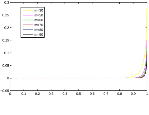
Figure 3. Approximation solution for m = 30, 50, 60, 70, 80, 90 for Troesch,s Problem in this study.
0 0.1 0.2 0.3 0.4 0.5 0.6 0.7 0.8 0.9 1
−0.05 0 0.05 0.1 0.15 0.2 0.25 0.3
m=30 m=50 m=60 m=70 m=80 m=90
4. NUMERICAL RESULTS
In this section, the DE-Sinc-Galerkin method (DESG) was applied to solve Troesch,s problem for severalms. Besides, the obtained results are compared with the results of other methods in the literatures [3,5,6,26].
To apply the DE-Sinc -Galerkin method, we supposed that d = π
4, γ = 1, B = 1
therefore for different values of N, h = ln (
πN 4
)
guessC0 as zero vector then use the Newton iteration (3.27). The last row in these tables is Maximum Error (MR) on top of that column.
In Tables 1 and 2, the exact solutions form= 0.5 andm= 1, and the numerical results of the present method are compared with some other existing methods includ-ing; decomposition method approximation (DMA) [3], modified homotopy perturba-tion method (HPM) [5], Sinc-Galerkin based on single exponential transformaperturba-tion (SESG) [26], and the Sinc-collocation method based on single exponential transfor-mation (SESC) [6]. It is interesting that inaccurate tabulated exact solutions are given in [3, 5, 6, 26]. If authors consider the exact solutions which is reported here and some other works [4, 8, 11], as a basis of comparison, they would have found that their approximation solutions were much more accurate than they realized in comparisons. In compare with the numerical results reported in some other work, the accuracy of the presented method is noticeable.
In Tables 3 and 4, absolute error in the solution of the Troesch,s Problem at
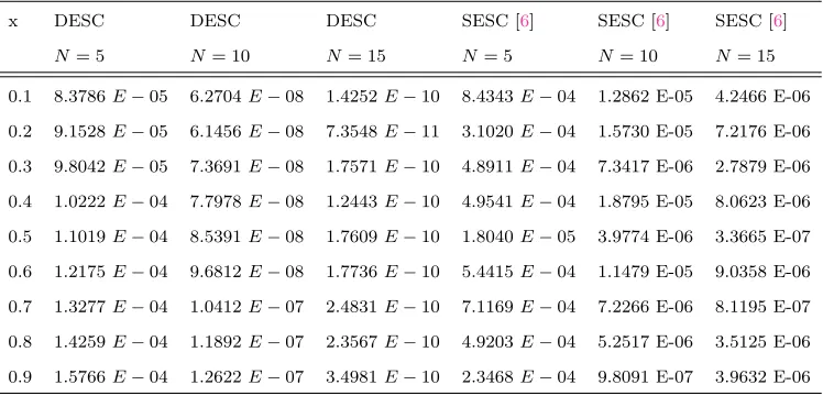
xj = 0.1,0.2, ...,0.9 with m = 0.5 and m = 1 are presented respectively. In these Tables, results of proposed method (DESG) for N = 5,10,15 and results of Sinc-collocation method based on single exponential (SESC) [6] for N = 5,10,15 are compared. These tables showed that the obtained results are more accurate than the results reported in Reference [6].
In Table 5 and 6, the comparison of our method with N = 5,10,15 and Sinc-Galerkin method based on single exponential transformation (SESG) [26] for N = 5,10,20 are tabulated. The results show that result of presented method are more accurate than Reference [26].
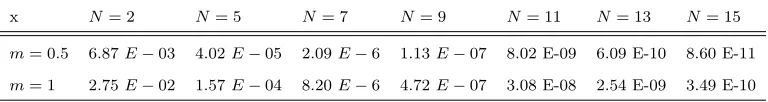
Table 7 shows the maximum absolute error in the solution at pointxj= 0.1,0.2,0.3, ...,0.9. Results of this table are demonstrated convergency of the method by increas-ing value of′N′.
Figure 1 displays solutions of DESG method form= 1,2,3, ...,10.
For m > 1 the decomposition method referenced in [3], Laplace decomposition method presented in [10] and B-Spline method in [9] do not yield a good approxi-mation. Although Khuri et al. [9] by using a few mesh points obtained appropriate results by B-Spline method, but using Sinc method without any changes given accept-able results. In Taccept-able 8 the numerical solution is calculated by DESG form= 5 and compared with numerical approximate of the exact solution given by a FORTRAN code called TWDBVP, the numerical solution of SESG [6] and B-spline method [9]
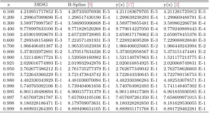
Beside, Figure 2 shows solution of DESG method form= 12,14,16,18,20. In Table 9 the numerical solution of DESG method by considerationN = 80 mesh points and adaptive collocation method given in [9] byN = 330 and numerical results obtained by Chang and Chang [2], and those obtained by Scott [17] form= 10 are compared.
Table 1. Results of Troesch,s Problem atm= 0.5.
x Exact Solution DESG DMA [3] HPM [5] SESG [26] SESC [6]
N= 15 N= 20 N= 20
0.1 0.0959443493 0.09594434932 0.09593835 0.09593956 ——- 0.0959445348
0.2 0.1921287477 0.19212874768 0.19211805 0.19211932 0.19212882 0.1921287458
0.3 0.2887944009 0.28879440094 0.28878032 0.28878069 ——- 0.2887947251
0.4 0.3861848464 0.38618484638 0.38616870 0.38616754 0.38618437 0.3861843754
0.5 0.4845471647 0.48454716477 0.48453029 0.48452741 ——- 0.4845471259
0.6 0.5841332484 0.58413324848 0.58411697 0.58411278 0.58413371 0.5841336720
0.7 0.6852011483 0.68520114831 0.68518684 0.68518224 ——- 0.6852009802
0.8 0.7880165227 0.78801652269 0.78800556 0.78800183 0.78801652 0.7880164746
0.9 0.8928542161 0.89285421616 0.89284802 0.89284621 ——- 0.8928542003
ME 8.60E−011 1.68E−005 2.04E−005 4.76 E-007 4.71 E-007
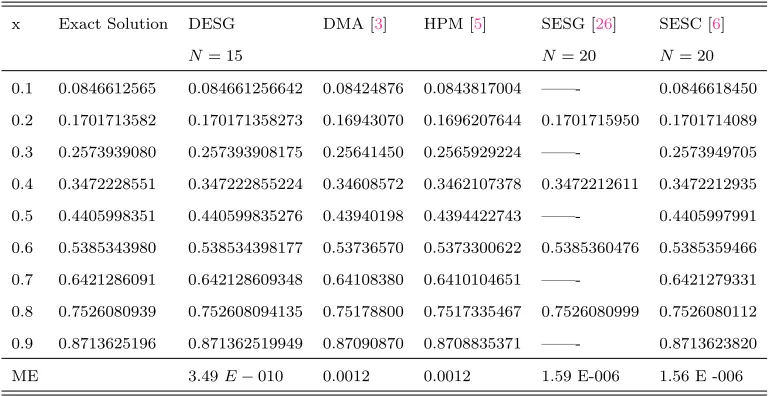
Table 2. Results of Troesch,s Problem at m= 1.
x Exact Solution DESG DMA [3] HPM [5] SESG [26] SESC [6]
N= 15 N= 20 N= 20
0.1 0.0846612565 0.084661256642 0.08424876 0.0843817004 ——- 0.0846618450
0.2 0.1701713582 0.170171358273 0.16943070 0.1696207644 0.1701715950 0.1701714089
0.3 0.2573939080 0.257393908175 0.25641450 0.2565929224 ——- 0.2573949705
0.4 0.3472228551 0.347222855224 0.34608572 0.3462107378 0.3472212611 0.3472212935
0.5 0.4405998351 0.440599835276 0.43940198 0.4394422743 ——- 0.4405997991
0.6 0.5385343980 0.538534398177 0.53736570 0.5373300622 0.5385360476 0.5385359466
0.7 0.6421286091 0.642128609348 0.64108380 0.6410104651 ——- 0.6421279331
0.8 0.7526080939 0.752608094135 0.75178800 0.7517335467 0.7526080999 0.7526080112
0.9 0.8713625196 0.871362519949 0.87090870 0.8708835371 ——- 0.8713623820
Table 3. Absolute error in the solution of Troesch,s Problem for
m= 0.5.
x DESG DESG DESG SESC [6] SESC [6] SESC [6]
N= 5 N= 10 N= 15 N= 5 N= 10 N= 15
0.1 2.2592E−05 1.8115E−08 2.5048E−11 2.3572E−04 1.2862 E-05 1.2652 E-06
0.2 2.5630E−05 1.6427E−08 1.7526E−11 9.2361E−05 1.5730 E-05 2.1638 E-06
0.3 2.7692E−05 2.3845E−08 4.3191E−11 1.2592E−04 7.3417 E-06 9.2352 E-07
0.4 2.8415E−05 1.7477E−08 1.5468E−11 1.3288E−04 1.8795 E-05 2.2513 E-06
0.5 3.0812E−05 2.5432E−08 7.4792E−11 4.1831E−06 3.9774 E-06 3.8266 E-08
0.6 3.3690E−05 3.1650E−08 8.6008E−11 1.2856E−04 1.1479 E-05 2.4579 E-06
0.7 3.5689E−05 2.4687E−08 1.0786E−11 1.7766E−04 7.2266 E-06 4.2468 E-07
0.8 3.7312E−05 3.4867E−08 7.2489E−12 1.4500E−04 5.2517 E-06 7.6033 E-07
0.9 4.0225E−05 3.0881E−08 6.4269E−11 9.1385E−05 9.8091 E-07 9.2200 E-07
Table 4. Absolute error in the solution of Troesch,s Problem for
m= 1.
x DESC DESC DESC SESC [6] SESC [6] SESC [6]
N= 5 N= 10 N= 15 N= 5 N= 10 N= 15
0.1 8.3786E−05 6.2704E−08 1.4252E−10 8.4343E−04 1.2862 E-05 4.2466 E-06
0.2 9.1528E−05 6.1456E−08 7.3548E−11 3.1020E−04 1.5730 E-05 7.2176 E-06
0.3 9.8042E−05 7.3691E−08 1.7571E−10 4.8911E−04 7.3417 E-06 2.7879 E-06
0.4 1.0222E−04 7.7978E−08 1.2443E−10 4.9541E−04 1.8795 E-05 8.0623 E-06
0.5 1.1019E−04 8.5391E−08 1.7609E−10 1.8040E−05 3.9774 E-06 3.3665 E-07
0.6 1.2175E−04 9.6812E−08 1.7736E−10 5.4415E−04 1.1479 E-05 9.0358 E-06
0.7 1.3277E−04 1.0412E−07 2.4831E−10 7.1169E−04 7.2266 E-06 8.1195 E-07
0.8 1.4259E−04 1.1892E−07 2.3567E−10 4.9203E−04 5.2517 E-06 3.5125 E-06
Table 5. Absolute error of DESG method for solution of Troesch,s Problem form= 0.5.
x DESG DESG DESG SESG [26] SESG [26] SESG [26]
N= 5 N= 10 N= 15 N= 5 N= 10 N= 20
0.2 2.5630E−05 1.6427E−08 1.7526E−11 1.7798E−05 1.7132 E-05 7.2300 E-08
0.4 2.8415E−05 1.7477E−08 1.5468E−11 1.5723E−04 1.6366 E-05 4.7640 E-07
0.6 3.3690E−05 3.1650E−08 8.6008E−11 1.1858E−04 1.5162 E-05 4.6160 E-07
0.8 3.7312E−05 3.4867E−08 7.2489E−12 5.0917E−05 5.1927 E-06 2.7000 E-09
Table 6. Absolute error in the solution of Troesch,s Problem for
m= 1.
x DESG DESC DESC SESG [26] SESG [26] SESG [26]
N= 5 N= 10 N= 15 N= 5 N= 10 N= 20
0.2 9.1528E−05 6.1456E−08 7.3548E−11 5.9688E−05 6.0723 E-05 2.3680 E-07
0.4 1.0222E−04 7.7978E−08 1.2443E−10 5.7321E−04 5.9727 E-05 1.5940 E-06
0.6 1.2175E−04 9.6812E−08 1.7736E−10 5.2725E−04 6.0328 E-05 1.6496 E-06
0.8 1.4259E−04 1.1892E−07 2.3567E−10 1.9061E−04 2.6693 E-05 6.0000 E-09
Table 7. Maximum Absolute Error in the solution for DE Sinc Galerkin method
x N= 2 N= 5 N= 7 N= 9 N= 11 N= 13 N= 15
m= 0.5 6.87E−03 4.02E−05 2.09E−6 1.13E−07 8.02 E-09 6.09 E-10 8.60 E-11
Table 8. Numerical solution of Troesch,s Problem form= 5
x DESG FORT.code [6] SESC [6] B-Spline [9]
0.2 0.01075340 0.01075342 0.00762552 0.01002027
0.4 0.03320049 0.03320051 0.03817903 0.03099793
0.8 0.25821648 0.25821664 0.23252435 0.24170496
0.9 0.45506002 0.45506034 0.44624551 0.42461830
Table 9. Numerical solution of Troesch,s Problem form= 10
x DESG B-Spline [9] y(x) [17] y(x) [2]
0.100 4.210951717852 E-5 4.207335076936 E-5 4.211183679705 E-5 4.211281725912 E-5 0.200 1.299647099690 E-4 1.298517430190 E-4 1.299639238293 E-4 1.299669488791 E-4 0.300 3.589779987567 E-4 3.586905006808 E-4 3.589778855481 E-4 3.589862266738 E-4 0.400 9.778997633100 E-4 9.771828520268 E-4 9.779014227050 E-4 9.779240889443 E-4 0.500 2.659019959670 E-3 2.657239728995 E-3 2.659017178062 E-3 2.659078455376 E-3 0.600 7.289348154660 E-3 7.224571491931 E-3 7.228924695208 E-3 7.229088828840 E-3 0.700 1.966406491387 E-2 1.965351623938 E-2 1.966406025665 E-2 1.966449243994 E-2 0.800 5.373032972891 E-2 5.370517634226 E-2 5.373032958567 E-2 5.373151474481 E-2 0.900 1.521140817724 E-1 1.520568160982 E-1 1.521140787863 E-1 1.521177213775 E-1 0.925 2.020016774993 E-1 2.019932942876 E-1 2.020016854925 E-1 2.020068749831 E-1 0.950 2.762677386212 E-1 2.761735277379 E-1 2.762677349042 E-1 2.762758626603 E-1 0.970 3.722643366229 E-1 3.721473843742 E-1 3.722643330645 E-1 3.722780156753 E-1 0.980 4.482330343929 E-1 4.481030070094 E-1 4.482330386284 E-1 4.482533078571 E-1 0.990 5.740765092106 E-1 5.739404061656 E-1 5.740764982493 E-1 5.741148407302 E-1 0.995 6.901149480694 E-1 6.900157731379 E-1 6.901149417369 E-1 6.901835930585 E-1 0.997 7.657697281787 E-1 7.657004105106 E-1 7.657697261350 E-1 7.658699971015 E-1 0.998 8.180328186471 E-1 8.179769073631 E-1 8.180328282850 E-1 8.181629530055 E-1 0.999 8.889931264395 E-1 8.889496654105 E-1 8.889931171768 E-1 8.891729462281 E-1
5. Conclusions
References
[1] S. Chang, Numerical solution of Troeschs problem by simple shooting method, Appl. Math. Comput.,216(2010), 3303-3306.
[2] S. H. Chang and I. L. Chang,A new algorithm for calculating the one-dimensional differential transform of nonlinear functions, Appl. Math. Comput.,195(2008), 799-808.
[3] E. Deeba, S. A. Khuri, and S. Xie,An algorithm for solving boundary value problems, J. Comput. Phys.,159(2000), 125-138.
[4] U. Erdoghan and T. Ozis,A smart nonstandard finite difference scheme for second order non-linear boundary value problems, J. Comput. Phys.,230(2011), 6464-6474.
[5] X. Feng, L. Mei, and G. He,An efficient algorithm for solving Troesch,s problem, Appl. Math.
Comput.,189(2007), 500-507.
[6] M. EL-Gamel, Numerical Solution of Troeschs Problem by Sinc-Collocation Method, Applied Mathematics,4(2013), 707–712.
[7] D. Gidaspow and B. S. Baker,A model for discharge of storage batteries, J. Electrochem. Soc.,
120(1973), 1005-1010.
[8] I. O. Govrilyuk, I. I. Lazurchak, and V. L. Mokarav,A method with a controllable exponential convergence rate for nonlinear differential operator equations, Comput. Meth. Appl. Math. 9
(2009), 63-78.
[9] S. A. Khuri and A. Sayfy,Troesch,s problem: A B-Spline collocation approach, Math. Comput.
Model.,54(2011), 1907–1918.
[10] S. A. Khuri,A numerical algorithm for solving the Troeschs problem, Int. J. Comput. Math.,
80(2003), 493-498.
[11] Y. Lin, J. A. Enszer, and M. A. Stadtherr,Enclosing all solutions of two point boundary value problems for ODEs, Comput. Chem. Eng.,32(2008), 1714-1725.
[12] J. Lund and K. Bowers,Sinc methods for quadrature and differential equation, SIAM , Philadel-phia , PA, 1992.
[13] V. S. Markin, A. A. Chernenko, Y. A. Chizmadehev, and Y. G. Chirkov,Aspects of the theory of gas porous electrodes, in: V.S. Bagotskii, Y.B. Vasilev (Eds.), Fuel Cells: Their Electrochemical Kinetics, Consultants Bureau, New York, 1966, 21-33.
[14] J. Rashidinia and M. Nabati,Sinc-Galerkin and Sinc-Collocation methods in the solution of nonlinear two-point boundary value problems. Comp. Appl. Math.,32(2013), 315–330. [15] S. M. Roberts and J. S. Shipman,On the closed form solution of Troesch,s problem, J. Comput.
Phys.,21(1976), 291-304.
[16] A. Saadatmandi, T. Abdolahi-Niasar,Numerical solution of Troesch,s problem using Christov rational functions, Computational Methods for Differential Equations,3(2015), 247-257. [17] M. R. Scott,On the conversion of boundary-value problems into stable initial-value problems via
several invariant imbedding algorithms, in: A.K. Aziz (Ed.), Numerical Solutions of Boundary-Value Problems for Ordinary Differential Equations, Academic Press, New York, 1975, 89-146 [18] F. Stenger,A Sinc-Galerkin method of solution of boundary value problems, J. Math. Comp.,
33(1979), 85–109.
[19] F. Stenger,Numerical method based on Sinc and analytic function, Springer-Verlag New York, 1993.
[20] M. Sugihara,Optimality of the double exponential formula- functional analysis approch, Numer. Math.,75(1997), 379–395.
[21] M. Sugihara,Near optimality of Sinc approximation, Math. Comput.,72(2003), 767–786. [22] H. Takahasi and M. Mori,Double exponential formulas for numerical integration, Publ. Res.
Inst. Math. Sci.,9(1974), 721–741.
[23] K. Tanaka, M. Sugihara, and K. Murata,Function classes for successful DE-Sinc approxima-tions, Math. Comput.,78(2009), 1553–1571.
[24] B. A. Troesch, Intrinsic difficulties in the numerical solution of a boundary value problem, Internal Report NN142, TRW Inc., Redondo Beach, California, 1960.
[26] M. Zarebnia and M. Sajjadian,The Sinc Galerkin method for solving Troesch,s problem, Math.