Solving high-order partial differential equations in unbounded
do-mains by means of double exponential second kind Chebyshev
ap-proximation
Mohamed Abdel-Latif Ramadan Mathematics Department, Faculty of Science, Menoufia University, Shebein El-Koom, Egypt. E-mail: [email protected]
Kamal Mohamed Raslan
Mathematics Department, Faculty of Science, Al-Azhar University, Nasr-City, Cairo, Egypt. E-mail: kamal [email protected]
Talaat El-Sayed El-Danaf
Department of Mathematics and Statistics, Taibah University Madinah Munawwarah, KSA. E-mail: [email protected]
Mohamed Ahmed Abd El Salam∗ Mathematics Department, Faculty of Science, Al-Azhar University, Nasr-City, Cairo, Egypt. E-mail: mohamed [email protected]
Abstract In this paper, a collocation method for solving high-order linear partial differential equations (PDEs) with variable coefficients under more general form of conditions is presented. This method is based on the approximation of the truncated double expo-nential second kind Chebyshev (ESC) series. The definition of the partial derivative is presented and derived as new operational matrices of derivatives. All principles and properties of the ESC functions are derived and introduced by us as a new basis defined in the whole range. The method transforms the PDEs and conditions into block matrix equations, which correspond to system of linear algebraic equations with unknown ESC coefficients, by using ESC collocation points. Combining these matrix equations and then solving the system yield the ESC coefficients of the solu-tion funcsolu-tion. Numerical examples are included to test the validity and applicability of the method.
Keywords. Exponential second kind Chebyshev functions, High-order partial differential equations, Col-location method.
2010 Mathematics Subject Classification. 65N04, 35G06.
Received: 30 December 2015 ; Accepted: 1 May 2016.
∗Corresponding author.
1. Introduction
It is well known that the numerical methods have played an important role in solving PDEs. Some of the well-known numerical methods are finite differences and finite element methods [6,17]. Recently, various approximate methods were discussed, such as differential transform method, Adomian decomposition method and Homo-topy analysis method [3,8,11,13,15,18]. Furthermore, spectral methods are one of the principal methods for solving differential equations. The main idea of spectral meth-ods is to approximate the solutions of differential equations by means of truncated series of orthogonal polynomials. The most used versions of spectral methods are tau, collocation, and Galerkin methods [1,5,9]. One of the most important orthogo-nal polynomials is Chebyshev polynomials. The well-known Chebyshev polynomials of the second kind Un(x) [12] are orthogonal with respect to the weight-function w(x) =√1−x2on the interval [−1,1], and the recurrence relation is
U0(x) = 1, U1(x) = 2x, Un+1(x) = 2xUn(x)−Un−1(x), n≥1.
Many studies of Chebyshev polynomials are considered on the first kindTn(x). On the other hand, in [10] and [14] a modified type of Chebyshev polynomials was proposed as new alternative technique to the solutions of ordinary and partial differential equa-tions given in whole domain. In their studies, the basis funcequa-tions called exponential Chebyshev functions, which are orthogonal on (−∞,∞) and are defined by
En(x) =Tn
ex−1 ex+ 1
,
2. Properties of double ESC functions
We introduce the definition of expotennial second kind Chebyshev ESC to be of the form
EUn(x) =Un
ex−1 ex+ 1
, (2.1)
where the corresponding recurrencs relation is
EU0(x) = 1, E1U(x) = 2
ex−1 ex+ 1
,
EUn+1(x) = 2
ex−1 ex+ 1
EnU(x)−EUn−1(x).
In Basu [4], the expression Tr,s(x, y) = Tr(x)·Ts(y) has given which is a form of Chebyshev polynomials. Mason et al. [12] have also used double Chebyshev polyno-mials expression for an infinitely differentiable functionu(x, y) defined on the square S(−∞< x, y < ∞), where Tr(x) andTs(y) are Chebyshev polynomials of the first kind. Now we employ our new definitionEnU(x) to double form.
Definition 2.1. The double ESC functions are in the following form
EUr,s(x, y) =ErU(x)·EsU(y), (2.2)
and the recurrence relation takes the form
EU
r+1,s(x, y) =
n
2eexx−1+1
EU
r(x)−ErU−1(x) o
·EU
s(y), r≥1, EU
r,s+1(x, y) =ErU(x)·
n
2eeyy−1+1
EU
s(y)−EsU−1(y) o
, s≥1.
(2.3)
2.1. Orthogonality of double ESC functions. The functions Er,sU (x, y) are or-thogonal with respect to the weight function
w(x, y) = 4e 3
2(x+y)(ex+ 1)−3 (ey+ 1)−3 ,
with the orthognality condition
Z ∞
−∞ Z ∞
−∞
Ei,jU(x, y)Ek,lU (x, y)w(x, y)dxdy=
π2
4 , i=j andk=l, 0, otherwise.
Also the product relation of double ESC functions used in the partial derivatives relations is given by
ex−1 ex+ 1
ey−1 ey+ 1
Em,nU (x, y) = 1 4[E
U
m+1,n+1(x, y) +E
U
m+1,n−1(x, y)
+EmU−1,n+1(x, y) +EmU−1,n−1(x, y)].
2.2. Function expansion in terms of double ESC functions. A functionu(x, y) well defined over the squareS(−∞< x, y <∞), can be expanded as
u(x, y) =
∞ X
r=0 ∞ X
s=0
ar,sEr,sU (x, y), (2.5)
where
ar,s = 4 π2
Z ∞
−∞ Z ∞
−∞
u(x, y)Er,sU (x, y)w(x, y)dxdy.
Ifu(x, y) in expression (2.5) is truncated to n, m < ∞in terms of the double ESC functions then, it will takes the form
U(x, y) = m
X
r=0
n
X
s=0
ar,sEr,sU (x, y),=E(x, y)·A, (2.6)
whereE(x, y) is 1×(m+1)(n+1) vector with elementsEU
r,s(x, y) andAis an unknown coefficient column vector, where
E(x, y) = [E0U,0(x, y) E0U,1(x, y) ... E0U,n(x, y)E1U,0(x, y) E1U,1(x, y) ...
E1U,n(x, y)... Em,U 0(x, y) Em,U 1(x, y) ... Em,nU (x, y)],
(2.7)
and
A= [a0,0 a0,1 ... a0,n a1,0 a1,1 ... a1,n ... am,0 am,1 .... am,n]T. (2.8)
2.3. The partial derivatives of double ESC functions. The operational matrices of derivatives of the double ESC functions are given in the next proposition
Proposition 2.2. The relation between the row vector E(x, y) and its (i,j)th-order partial derivative is given as
where, Dx andDy are the(m+ 1)(n+ 1)×(m+ 1)(n+ 1)operational matrices for the partial derivatives, and the general form of them is
Dx=diag
α
4 + 1 2γα
I, 0, −α 4 I
T
,
α = 0, 1, ..., m, γα=
(
0, ifα= 0, 1, ifα6= 0,
(2.10)
and
Dy =
η 0 · · · 0 0 η · · · 0 ..
. ... . .. ...
0 0 · · · η
T
, η=diag
β
4 + 1 2γβ, 0,
−β 4
,
β = 0, 1, ..., n, γβ=
(
0, if β= 0, 1, if β6= 0,
(2.11)
whereIand0are(n+ 1)×(n+ 1) identity and zero matrices in the block matrixDx which is(m+ 1)×(m+ 1). Alsoη is the matrix of (n+ 1)×(n+ 1) in the block matrixDy which is(m+ 1)×(m+ 1).
Proof. The partial derivatives of the ESC functions can be obtained by differentiating relation (2.3), first with respect to the variablex,and with the help of (2.6) we get
∂ ∂x E
U
0,s(x, y)
= 0, for alls, (2.12)
∂ ∂x E
U
1,s(x, y)
= 4ex
(1+ex)2E U
s(y) = 34E
U
0(x)−14E
U 2(x) EU s(y) = 3 4E U
0,s(x, y)−14E
U
2,s(x, y),
(2.13)
and
∂ ∂x E
U
r+1,s(x, y)
= ∂ ∂x
2EU
1,s(x, y)Er,sU (x, y)−EUr−1,s(x, y)
= ∂ ∂x
h
2 EU
1,s(x, y)
(0,0)
EU r,s(x, y)
(0,0)
− EU
r−1,s(x, y)
(0,0)i
= [2 EU
1,s(x, y)
(1,0)
EU r,s(x, y)
(0,0)
+ 2 EU
1,s(x, y)
(0,0)
EU r,s(x, y)
(1,0)
− ErU−1,s(x, y)
(1,0)
],
by using the relations (2.12)-(2.14) and with the help of product relation for r = 0,1, ..., m, the elements of the matrix of dersvatives Dx can be obtained from the following equalities EU
0,s(x, y)
(1,0)
= 0,
E1U,s(x, y)(1,0)= 34E0U,s(x, y)−1 4E
U
2,s(x, y), EU
2,s(x, y)
(1,0)
=EU
1,s(x, y)−12E
U
3,s(x, y), ..
. EU
r,s(x, y)
(1,0)
=r+24 Er−1,s(x, y)−r4Er+1,s(x, y), r >1, for alls. (2.15)
Similarly, we get the partial derivative with respect to the variabley as
EU r,0(x, y)
(0,1)
= 0,
Er,U1(x, y) (0,1)
=34Er,U0(x, y)−14E
U r,2(x, y),
EU r,2(x, y)
(0,1)
=EU
r,1(x, y)− 1 2E
U r,3(x, y),
.. .
EU r,s(x, y)
(0,1)
=s+24 Er,s−1(x, y)−s4Er,s+1(x, y), s >1, for allr.
(2.16)
Then, the previous equalities (2.15),(2.16) form (m+ 1)(n+ 1)×(m+ 1)(n+ 1) two operational matricesDx andDy by our consideration that
Er,sU (x, y)(1,0)= EUr,s(x, y)(0,1)= EUr,s(x, y)(0,0)= 0, forr > mands > n.
Thus, to obtain the matrixE(i,j)(x, y) in terms of E(x, y), we can use the relation (2.15), (2.16) as
E(1,0)(x, y) =E(x, y)Dx,
E(2,0)(x, y) =E(1,0)(x, y)Dx= (E(x, y)Dx)Dx=E(x, y) (Dx)
2
,
E(3,0)(x, y) =E(1,0)(x, y) (Dx,)2=E(x, y) (Dx)3. Therefore, by induction we can write
E(i,0)(x, y) =E(x, y) (Dx) i
, (2.17)
similarly
hence, by using (2.17), (2.18) we get finally
E(i,j)(x, y) =E(x, y) (Dx) i
(Dy) j
, (2.19)
which end the proof.
3. Application of the introduced partial derivatives for high-order
PDEs
The forms of high-order linear non-homogeneous partial differential equations with variable coefficients in unbounded domains are
p
X
i=0
r
X
j=0
qi,j(x, y)u(i,j)(x, y) =f(x, y),−∞< x, y <∞, (3.1)
with the non-local conditions [7], [16]
ρ
X
t=1
p
X
i=0
r
X
j=0
bti,ju(i,j)(ωt, ηt) =λ ,
and / or
ν
X
t=1
p
X
i=0
r
X
j=0
cti,j(x)u(i,j)(x, γt) =g(x), (3.2)
and / or
θ
X
t=1
p
X
i=0
r
X
j=0
dti,j(y)u(i,j)(εt, y) =h(y),
where the u(0,0)(x, y) = u(x, y), u(i,j)(x, y) = ∂x∂ii+∂yjju(x, y) and qi,j(x, y), f(x, y), ct
i,j(x),g(x),dti,j(y) andh(y) are known functions on the squareS(−∞< x, y <∞,), andωt, ηt,γt,εtare constants∈ (−∞,∞) and may be one or more of them tends to infinity. Now, we consider that the approximate solutionU(x, y) to the exact solution u(x, y) of Eq. (3.1) defined by expression (2.6) and its (i, j)-th partial derivatives defined by Eq. (2.19) as
U(x, y) = m
X
r=0
n
X
s=0
ar,sEr,s(x, y) =E(x, y)·A, (3.3)
and
4. Fundamental matrix relations
Let us define the collocation points [10,14], so that−∞< xi, yi<∞,as
xk=Ln
1+cos(kπ
m)
1−cos(kπ
m)
, yl=Ln
1+cos(lπ
n)
1−cos(lπ
n)
,
(k= 1, ..., m−1, l= 1, ..., n−1)
(4.1)
and at the boundaries
(k= 0, k=m) x0→ ∞, xm→ −∞,(l= 0, l=n)y0→ ∞, yn → −∞.
Since the double ESC functions are convergent at both boundaries ±∞, then the appearance of infinity in the collocation points does not cause a loss or divergence in the method. Now, we substitute the collocation points (4.1) into Eq. (3.1) to obtain
p X i=0 r X j=0
qi,j(xk, yl)u(i,j)(xk, yl) =f(xk, yl), (4.2)
the system (4.2) can be written in the matrix form
p X i=0 r X j=0
Qi,j U(i,j)=F, p≤m, r≤n, (4.3)
where Qi,j denotes the diagonal matrix with inner elements are qi,j(xk, yl) where, (k = 0,1,2, ..., m;l = 0,1,2, ..., n) and F denotes the column matrix with the elementsf(xk, yl) where, (k= 0,1,2, ..., m;l = 0,1,2, ..., n), by substituting the collocation points (4.1) into derivatives of the unknown function as in Eq. (3.4) yields
U(i,j)=
U(i,j)(x 0, y0)
.. . U(i,j)(x0, yn) U(i,j)(x
1, y0)
.. . U(i,j)(x
1, yn) .. . U(i,j)(x
n, ym)
= [E(Dx)i(Dy)j]A , (4.4)
where
therefore, from Eq. (4.3), we get a system of matrix equation ”fundamental matrix” for the PDE in the following form
p
X
i=0
r
X
j=0 Qi,j
E(x, y)(Dx)i(Dy)j
A =F, (4.5)
which corresponds to a system of (m+ 1)(n+ 1) linear algebraic equations with (m+ 1)(n+ 1) double ESC coefficientsar,sunknowns. By substituting the collocation points (4.1) in the condition (3.2) by same procedure before we get the fundamental matrices for conditions as
Pρ
t=1 Pp
i=0 Pr
j=0bti,j
E(ωt, ηt) (Dx)i(Dy)j A=λ,
Pν
t=1 Pp
i=0 Pr
j=0c
t i,j(xk)
E(xk, γt) (Dx)i(Dy)j A=g(xk),
Pθ
t=1 Pp
i=0 Pr
j=0d
t i,j(yl)
E(εt, yl) (Dx)i(Dy)j A=h(yl).
(4.6)
It is also noted that the structure of matricesQi,jandFvary according to the number of collocation points and the structure of the problem. However, E, Dx and Dy do not change their nature for fixed values ofmandnwhich are truncation limits of the ESC series. In the other words, the changes inE,DxandDy are only dependent on the number of collocation points.
5. Method of solution
The fundamental matrix (4.5) for Eq. (3.1) corresponding to a system of (m+1)(n+ 1) algebraic equations for the (m+1)(n+1) unknown ESC coefficientsa0,0, a0,1,· · · , a0,n, a1,0, a1,1,· · · , a1,n,· · · , am,0, am,1,· · · , am,n.
We can write the matrix (4.5) as
WA=F, or [W; F], (5.1)
and we can obtain the matrix form for the conditions by means of (4.6) in a compact form as
VA=R, or [V;R], (5.2)
whereVis ah×(m+ 1)(n+ 1) matrix andRis ah×1 matrix, so thathis the rank of the all row matrices as in (4.6) belong to the given conditions. Then (5.1) together with (5.2) can be written in the following compact form:
W∗A=F∗, or [W∗;F∗]. (5.3)
and thereforeW∗ becomes a rectangular matrix. To solve this new system, the gen-eralized inverse of W∗ can be used [7], and so the double ESC coefficients can be found as
A= geninv(W∗)·F∗.
The method procedure can be summarized by the following algorithm: 1. Calculating the matrixW;
2. Forming the matrixW∗ by addingV;
3. Solving the system of algebraic equations and finding ESC coefficients.
6. Test examples
We consider here some test examples that will be numerically treated by the above proposed method. The numerical computations are carried out by the Mathematica. 7.0.
Example: 6.1
Consider the following partial differential equation
u(2,1)+ 1 1 +exu
(1,0)=f(x, y), x, y∈(−∞, ∞), (6.1)
to be the first test problem, with exact solution
u(x, y) = (−5 + 3Coshy)Sech2y
2 T anh x 2
,
where, the functionf(x, y) takes the form
f(x, y) = Sech
2 x
2
−5 + 3Coshy−8(−1 +ex)T anh x2 (−1 +ex)(1 +Coshy) , and the subjected conditions are
u(x, y) = 6T anh x2
, at y→ ∞,
u(x, y) = 6 at x→ ∞ and at y→ −∞, u(0,0) = 0,
u(x,0) = 2 at x→ −∞.
The fundamental matrix takes the form
n
Q1,0hE(Dx)1i+Q2,1hE(Dx)2(Dy)1ioA=F,
we takem=n= 8, where, the approximate solution given by
Then, after the augmented matrix of the system and conditions are computed, we obtain the coefficients solution as:
a0,0= a0,1= ... =a0,8= 0,
a1,0= 0, a1,1= 0, a1,2= 1, ..., a1,8= 0,
a2,0= a2,1=... =a2,8= 0,
.. .
a8,0= a8,1= ...= a8,8= 0,
and the solution is given as: U(x, y) =EU
1,2(x, y),
U(x, y) = 2eexx−1+1
−1 + 4ey−1
ey+1
2
= (−5 + 3Coshy)Sech2y
2
T anh x2
,
which represent the exact solution of the problem.
Example: 6.2
Consider the following differential equation [10]
uxy− 2 1 +exuy=
4ey
(1 +ex)2(1 +ey)2, x, y ∈(−∞, ∞), (6.2)
with conditions
uy(0, y) = 0, u(x,0) = 0.
The fundamental matrix takes the form
n
Q0,1hE(Dy)1i+Q1,1hE(Dx)1(Dy)1ioA=F,
we takem=n= 4, where the approximate solution given by
U(x, y) =a0,0E0U,0(x, y) +a0,1E0U,1(x, y) +· · ·+a4,4E4U,4(x, y),
then, after the augmented matrix of the system and conditions are computed, we obtain the coefficients:
a0,0= a0,1= ... =a0,4= 0,
a1,0= 0, a1,1=14, a1,2=a1,3=a1,4= 0,
a2,0= a2,1= ... =a4,4= 0,
and the solution is given by: U(x, y) = 14EU
1,1(x, y), or
U(x, y) = 1 4
2
ex−1 ex+ 1
2
ey−1 ey+ 1
=
ex+y−ex−ey+ 1 (ex+ 1) (ey+ 1)
which represent the exact solution of Eq (6.2). On the other hand, the approximate solution given in [10] atn=m= 15 the approximate solution doesn’t give the exact solution.
Example: 6.3
The Cauchy problem [16], for the one-dimensional homogeneous wave equation is given by
uyy−c2uxx= 0, −∞< x <∞, y∈[0, ∞), u(x,0) =f(x), uy(x,0) =g(x), −∞< x <∞.
(6.3)
The solution of this problem can be interpreted as the amplitude of a sound wave propagating in very long and narrow pipe, which in practice can be considered as one-dimensional infinite medium. The initial conditionsf, gare given functions that represent the amplitudeu(x, y) and the velocity uy of the string at timey = 0. The exact solution of (6.3) is given by DAlemberts formula
u(x, y) = 1
2[f(x+cy) +f(x−cy)] + 1 2c
Z x+cy
x−cy
g(s)ds.
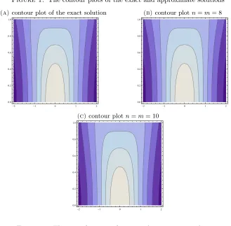
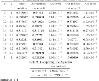
Thus, if we take f(x) = Sech(x) and g(x) = 0, and applying our present method to solve (6.3), at n = m = 8, and 10 by using double ESC collocation points, we obtain the approximate solution U(x, y). In Table 1, the exact and approximate solutions are listed according to different values ofx, y. The calculation of L2 norm
L2= q
hPI
i=0(ui−Ui) 2
Figure 1. The contour plots of the exact and approximate solutions
(a)contour plot of the exact solution
-2 -1 0 1 2
0.0 0.2 0.4 0.6 0.8 1.0
(b)contour plotn=m= 8
-2 -1 0 1 2
0.0 0.2 0.4 0.6 0.8 1.0
(c)contour plotn=m= 10
-2 -1 0 1 2
0.0 0.2 0.4 0.6 0.8 1.0
Figure 2. The error function of exact and approximate solutions
Table. 1 comparing the approximate and exact solution x y Exact Our method Abs error Our method Abs error
solution n=m= 8 n=m= 10
0 1 0.648054 0.64752 5.34×10⁻⁴ 0.647913 1.41×10⁻⁴
0.1 0.9 0.697877 0.697663 2.13×10⁻⁴ 0.697525 4.94×10⁻⁴
0.2 0.5 0.876667 0.877628 9.60×10⁻⁴ 0.874907 8.92×10⁻⁴
0.3 0.7 0.786531 0.787771 1.23×10⁻³ 0.786684 1.52×10⁻⁴
0.4 0.6 0.814191 0.816115 1.92×10⁻³ 0.815118 9.27×10⁻⁴
0.5 0.5 0.824027 0.826211 2.18×10⁻³ 0.825253 1.22×10⁻³
0.6 0.3 0.827211 0.828661 1.44×10⁻³ 0.82791 6.98×10⁻⁴
0.7 0.4 0.777981 0.77964 1.65×10⁻³ 0.778372 3.90×10⁻⁴
0.8 0.7 0.710058 0.710421 3.62×10⁻⁴ 0.710033 2.50×10⁻⁵
0.9 0.2 0.69802 0.697939 8.03×10⁻⁵ 0.697525 4.94×10⁻⁴
1 1 0.632901 0.631296 1.60×10⁻³ 0.63639 3.48×10⁻³
Table 2. Comparing theL2-norm
our method n=m= 8 1.04597×10⁻³
n=m= 10 4.16219×10⁻⁴
Example: 6.4
Let us consider the Poisson equation [2,16]
52u=f(x, y), 0≤x, y≤1. (6.4)
Poisson equation arises in steady state heat problems with time independent heat sources, where the Dirichlet boundary conditions in general form is
u(0, y) =f1(y), u(x,0) =g1(x),
u(1, y) =f2(y), u(x,1) =g2(x).
If we chose the exact solution to be as
u(x, y) = (1 +ex)−1(1 +ey)−1, then, we find
f1(y) =
1 2(1 +e
y)−1
, g1(x) =
1 2(1 +e
x)−1
,
f2(y) = (1 +ey)−1(1 +e)−1, g2(x) = (1 +e)−1(1 +ex)−1.
U(x, y) = 0.25EU0,0(x, y)−0.125E0U,1(x, y)−0.125EU
1,0(x, y) + 0.0625E
U
1,1(x, y).
By simplifying the previous relation we reach to
U(x, y) = (1 +ex)−1(1 +ey)−1,
which represent the exact solution of Poisson equation (6.4) with the connected con-ditions.
7. Conclusion
In this paper, a collocation method for solving high-order linear partial differential equations with variable coefficients under more general form of conditions is investi-gated. The method is based on the approximation by truncated double exponential second kind Chebyshev (ESC) series, and the definition of the partial derivatives is presented. All principles and properties of this type are derived and introduced by us as new definitions. The definition of the partial derivatives of ESC functions is presented and derived as new operational matrices of derivatives. The PDEs and conditions are transformed into block matrix equations, which correspond to system of linear algebraic equations with unknown ESC coefficients, by using ESC colloca-tion points. The generalized invers is used to solve this linear system and to find the ESC coefficients. Illustrative examples are used to demonstrate the applicability and the effectiveness of the proposed technique. In addition, an interesting feature of this method is to find the analytical exact solution if the equation has an exact solution of rational exponential form. The method can also be extended to high-order nonlin-ear partial differential equation with variable coefficients, but some modifications are required.
Acknowledgment
The authors sincerely thank the editors, reviewers and everyone who provide the advice, support, help and useful comments. The product of this research paper would not be possible without all of them.
References
[1] W. M. Abd-Elhameed, Y. H. Youssri and E. H. Doha,A novel operational matrix method based
on shifted Legendre polynomials for solving second-order boundary value problems involving
[2] N. H. Asmar, Partial differential equations with fourier series and boundary value problems, PERSON, Prentic Hall, 2004.
[3] A. Basiri Parsa, M. M. Rashidi, O. Anwar Bg and S.M. Sadri,Semi-computational simulation of
magneto-hemodynamic flow in a semi-porous channel using optimal Homotopy and differential transform methods, Computers in Biology and Medicine,43: 9(2013), 1142–1153.
[4] N. K. Basu,On double Chebyshev series approximation,SIAM J. Numer. Anal.,10: 3 (1973),
496–505.
[5] A. H. Bhrawy,An efficient Jacobi pseudo spectral approximation for nonlinear complex
gener-alized Zakharov system, Applied Math. and Comput.,247(2014), 30–46.
[6] R. L. Burden and J. D. Faires,Numerical analysis, Cengage Learning, 2011.
[7] A. Dascioglu,Chebyshev polynomial approximation for high-order partial differential equations with complicated conditions, Numer. methods for partial Differ. Equ.,25(2009), 610–621.
[8] E. Erfani, M. M. Rashidi, and A. Basiri Parsa,The modified differential transform method for
solving off-centered stagnation flow toward a rotating disc, Int. J. of Comput. methods, 7: 4
(2010) 655–670.
[9] B. Y. Guo, and J. P. Yan,LegendreGauss collocation method for initial value problems of second
order ordinary differential equations. Applied Numer. Math.,59(2009), 1386–1408.
[10] A. B. Koc and A. Kurnaz, A new kind of double Chebyshev polynomial approximation on
unbounded domains, Boundary value problems,2013: 1(2013), 1687–2770.
[11] S. J. Liao,Beyond perturbation: introduction to the Homotopy analysis method, CRC Press, Boca Raton: Chapman & Hall, 2003.
[12] J.C. Mason and D.C. Handscomb,Chebyshev polynomials, CRC Press, Boca Raton, 2003.
[13] A. A. Ragab, K. M. Hemida, M. S. Mohamed, and M. A. Abd El Salam,Solution of time-fractional Navier-Stokes equation by using Homotopy analysis method, Gen. Math. notes,13:
2(2012) 13–21.
[14] M. A. Ramadan, K. R. Raslan T. S. El Danaf and M. A. Abd El salam,On the exponential Chebyshev approximation in unbounded domains: A comparison study for solving high-order
ordinary differential equations, Int. J. of pure and applied Math.,105: 3(2015), 399–413.
[15] M. M. Rashidi, E. Momoniat, and B. Rostami, Analytic approximate solutions for MHD boundary-layer viscoelastic fluid flow over continuously moving stretching surface by homotopy
analysis method with two auxiliary parameters, J. of Applied Math.,2012(2012), 1–19.
[16] M. Sezer,A Chebyshev series approximation for linear second-order partial differential equa-tions with complicated condiequa-tions, Gazi Uni. J. of Sci.,26: 4(2013), 515–525.
[17] G. D. Smith,Numerical Solution of Partial Differential Equations, Clarendon Press, Oxford,
2005.