in the population sciences published by the Max Planck Institute for Demographic Research Konrad-Zuse Str. 1, D-18057 Rostock·GERMANY www.demographic-research.org
DEMOGRAPHIC RESEARCH
VOLUME 17, ARTICLE 3, PAGES 59-82
PUBLISHED 03 AUGUST 2007
http://www.demographic-research.org/Volumes/Vol17/3/ DOI: 10.4054/DemRes.2007.17.3
Research Article
The ”Wedding-Ring”:
An agent-based marriage model
based on social interaction
Francesco C. Billari
Alexia Prskawetz
Belinda Aparicio Diaz
Thomas Fent
c
°2007 Billari et al.
1. Introduction 60
2. Social interaction and marriage: Theory and hypotheses 63
3. An agent-based model: The “Wedding Ring” 64
4. Model implementation 68
5. Simulation results 71
6. Sensitivity analysis 73
7. Summary and discussion 75
The ”Wedding-Ring”:
An agent-based marriage model
based on social interaction
Francesco C. Billari1 Alexia Prskawetz2
Belinda Aparicio Diaz3 Thomas Fent4
Abstract
In this paper we develop an agent-based marriage model based on social interaction. We build an population of interacting agents whose chances of marrying depend on the avail-ability of partners, and whose willingness to marry depends on the share of relevant oth-ers in their social network who are already married. We then let the typical aggregate age pattern of marriage emerge from the bottom-up. The results of our simulation show that micro-level hypotheses founded on existing theory and evidence on social interaction can reproduce age-at-marriage patterns with both realistic shape and realistic micro-level dynamics.
1Carlo F. Dondena Center for Research on Social Dynamics, IGIER and Department of Decision Sciences,
Università Bocconi,Milan. E-mail: [email protected]
2Vienna Institute of Demography, Austrian Academy of Sciences, Vienna.
E-mail: [email protected]
3Vienna Institute of Demography, Austrian Academy of Sciences, Vienna.
E-mail: [email protected]
4Vienna Institute of Demography, Austrian Academy of Sciences, Vienna.
1. Introduction
In the social and behavioral sciences, the timing of marriage has been studied from two different perspectives. On the one side, demographers and sociologists have focused on explaining and modeling important stylized facts such as the typical shape of age–at– marriage curves; their analytical strategies have usually relied on mathematical and statis-tical macro–level models. On the other side, psychologists and economists have focused on studying and modeling the process of partner search; micro–level assumptions have usually been at the heart of this approach.
More recently, agent–based modeling has been proposed as a convenient approach to build models that account for macro–level marriage patterns while starting from plausi-ble micro–level assumptions. This is particularly important in marriage models because agent–based models allow for realistic hypotheses on the interaction between heteroge-neous potential partners that typically takes place in the marriage market (Billari et al., 2003; Todd and Billari, 2003; Simão and Todd, 2003; Todd et al., 2005; Aparicio Diaz and Fent, 2006). The study of the emergence of macro–level outcomes from micro–level models that contains social interactions allows to bridge the micro– and macro–level per-spective from “the bottom-up”. This approach is very widely used in agent–based mod-els, for which the application to demographic choices has been recently advocated (Billari and Prskawetz, 2003). The macro–level outcome that has been studied the most is the age pattern of marriage, which demographers have shown as being characterized by constant features over time and space (Coale, 1971; Coale and McNeil, 1972).
Partnership formation is by definition social interaction itself. In contemporary soci-eties, the great majority of potential partners meet each other, talk to each other, have sex before cohabiting or getting married. Nevertheless, important scientific evidence signals that social interactions taking place in the marriage market are not limited to those be-tween potential partners. Indeed, the study of the impact of what “relevant others” think and do on key decisions concerning our lives — such as getting married and having chil-dren — has emerged as an important field of research (Bongaarts and Watkins, 1996). Montgomery and Casterline (1996; 1998) identify two distinct processes through which relevant others matter: first, “social learning”, reflecting acquisition of information in a network; second, “social influence”, reflecting the power relevant others might exercise over an individual through authority, deference, and social conformity pressure. While most results on social learning and social influence refer to contraceptive and fertility choices in the developing world, recent evidence from qualitative surveys shows that both social learning and social influence are among the important factors in the decision to get married in a contemporary society (Bernardi, 2003).
assumption that a diffusion process takes place within a cohort of individuals, with the share of married “peers” influencing the propensity to marry. In the Hernes’ model case, the assumption is that members of the same cohort constitute the influential peer group. In the original Hernes paper, the assumption is mostly justified on the casual evidence of everyday life. In what follows, we join the essentially micro–level research tradition focusing on social interaction with the macro–level ideas pioneered by Hernes on age– at–marriage patterns. We refer to social interaction in general, although the role of social learning is likely to be more important than the role of social influence. We thus build a marriage model starting from the micro–level, including social interaction (or, as, we call it, “social pressure”) as the key force driving the marriage process.
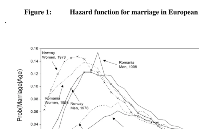
Our aim is to let the typical macro–level shape of age–at–marriage patterns emerge from the bottom-up, as an outcome of our assumptions on individual behavior and social interaction. More specifically, we assume that agents belonging to the social network of an agent — the “relevant others” — influence the desire of an individual to get married. The actual realization of such desire is mediated by the characteristics of the marriage market (i.e. the availability and location of potential partners). As two partners get married they start having children, and our model simulates the population dynamics that follows. Similarly to Todd and Billari (2003) and Todd et al. (2005), the macro–level outcome against which we test our model is the shape of the hazard of marriage, i.e. the age– specific probability of marrying conditional on not having married by a certain birthday. From various sources, we know that the hazard of marriage has an asymmetric non– monotonic shape. In addition, hazard rates tend to converge to a level close to zero at later ages. This curve has been modeled in various ways from a macro–level perspective. The most widespread models are the ones proposed by Coale and McNeil (Coale, 1971; Coale and McNeil, 1972) — see Kaneko (2003) for a recent generalization of the Coale-McNeil model — and by Hernes (1972). Figure 1. (from Todd et al., 2005) shows the empirically observed functions for men and women in three populations of the late twentieth century: Romania, 1998, and Norway, 1978 and 1998. In all the cases shown in the figure, the rise of age–specific probabilities is faster than its decrease. Although the shape of the curve looks rather different for Norway 1998, where non–marital cohabitation is widespread, it can still be described qualitatively in a similar way.
Figure 1: Hazard function for marriage in European populations
.
2. Social interaction and marriage: Theory and hypotheses
For a given individual, the set of “relevant others” consists of people who are close to her/him, i.e. the member of her/his “social network”. Closeness is a feature that can be modeled in a relatively straightforward way within an agent–based framework. In our context, the term “close” refers to a distance that may represent a spatial distance (i.e. neighbors are potential relevant others), but might as well represent a distance in terms of kinship, age, education, professional occupation, and so on. Closer individuals are more likely to get married: homogamy in marriage along various dimensions such as ethnicity, religion, socioeconomic status, and even attractiveness, intelligence, height has been clearly documented (Kalick and Hamilton, 1986; Kalmijn, 1998; Coltrane and Collins, 2001).
The size and characteristics of an individuals’ social network may vary with individ-uals’ characteristics. An important result is that the number of relevant others increases with age during youth and adulthood, at least up to ages that are important for processes such as getting married or having children, and decreases thereafter (Hammer et al., 1982; Marsden, 1987; Morgan, 1988; van Tilburg, 1995; Völker and Flap, 1995; van Tilburg, 1998; Due et al., 1999; Micheli, 2000; Wagner and Wolf, 2001).
If one needs to operationalize the importance of social interaction in the decision to get married, besides the mere effect of availability of a partner around oneself, we can look at how relevant others behave. The literature on social interaction has shown that relevant others provide information (i.e. social learning), and trigger normative influence (i.e. social influence). Both social learning and social influence might trigger the diffusion of marriage within a social network (Montgomery and Casterline, 1996; 1998). Normative pressure, as assumed by Hernes (1972) plays a key role especially as it might depend on an individual’s age. Moreover, if we assume that marriage makes people happy at least for a while (Clark and Oswald, 2002; Kohler et al., 2005), also social learning may trigger the same effect. It is therefore likely that the share of married people among the relevant others in one’s social network has a positive impact on an individuals’ desire to get married (Bernardi, 2003). This was the key assumption of the macro–level diffusion model developed by Hernes (1972).
the transmission of infectious diseases is that in case of marriage it is not sufficient to get “infected” by married people. A person who experiences a high level of pressure through social interaction and who might, as a consequence, intend to get married, also needs to find a partner who is not yet married. This partner will usually also be somebody within the individuals’ social network. Hence, the highest incidence of marriage occurs within a social network exhibiting a relatively high share of both married and unmarried persons. On the contrary, in case of an infectious disease an individual who is in contact with an almost entirely infected population (and who is susceptible) experiences the highest expo-sure to the risk of getting infected. An agent–based framework allows to fully incorporate the problem of finding an available partner within a diffusion approach.
Moreover, not only the share of married people within the social network, but also the time span since they got married might have an influence. This may be due to the fact that weddings that have just taken place may make a stronger impression within the social network than weddings that have taken place decades ago. We may mention three reasons to justify this idea. First, when a relevant other gets married, the wedding ceremony might trigger the desire to get married. Weddings are also occasions during which potential partners sometimes meet for the first time (as our own casual experience shows). Second, the increase in happiness related to marriage has been shown to slowly vanish over time (Clark and Oswald, 2002). Third, the information coming from married couples might become increasingly less relevant for single persons as the duration of marriage increases. Therefore, an unmarried person who has already been confronted with married people for a long time without getting actually married her– or himself may feel less pressure than an unmarried person witnessing the marriage of relevant others. Another aspect to be considered is the possibility of married people to get divorced, which may cause a negative attitude toward marriage within their social network. However, to model this effect we would need to model divorce in addition to marriage. In what follows we model first marriage as an irreversible process.
3. An agent-based model: The “Wedding Ring”
The agent-based model we develop builds on the ideas and hypotheses that have been discussed in previous sections. In our model, agents live in a world which is arranged along a circular line — due to the analogy with a wedding ring, this circle may also be called a ring. The model itself is thus called “Wedding Ring”.
the space. If we think about the spatial location of agents, a ring is a simple analogon to the real world, where we all live on a surface approximating a sphere. Approximat-ing the world by a rApproximat-ing may also be appropriate with respect to kinship and professional occupation.5
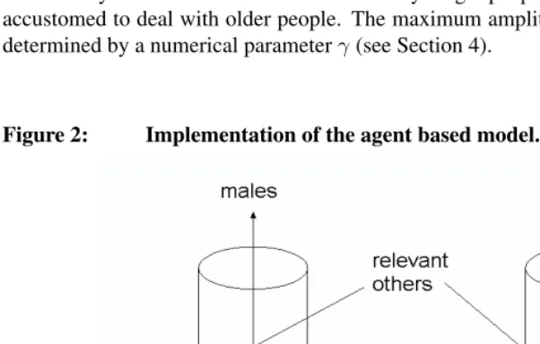
Our model uses a yearly time scale. We use age (in years)x, the main covariate in existing marriage models, as the second main coordinate of agents. We may therefore imagine the agents in our model as distributed within a space that can be regarded as the lateral surface of a circular cylinder (cf. Figure 2)—i.e. a ring with a height equal to the length of life.
We define the social network of relevant others as containing a random number of agents located within a two–dimensional neighborhood on this surface. This two–dimen-sional neighborhood is usually symmetric with respect to the agents spatial location. We also allow for asymmetric intervals with respect to age, reflecting the fact that some indi-viduals may be more accustomed to deal with younger people, while others may be more accustomed to deal with older people. The maximum amplitude of this heterogeneity is determined by a numerical parameterγ(see Section 4).
Figure 2: Implementation of the agent based model.
5However, a one–dimensional interval might be a better choice for modeling characteristics with a rank
The proportion of married people within the network of relevant others,pom, deter-mines the social interaction effect (for simplicity, we use the term “social pressure” to denote the effect of social interaction, including both social learning and social influence from now onwards). Social pressure is defined as a function ofpom:
sp= exp(β(pom−α))
1 + exp(β(pom−α)), (1)
whereαandβdetermine the inflection point and slope of the function (cf. Figure 3).
Figure 3: Functional form of social pressure.
0 0.1 0.2 0.3 0.4 0.5 0.6 0.7 0.8 0.9 1
0 0.1 0.2 0.3 0.4 0.5 0.6 0.7 0.8 0.9 1 pom
s
o
c
ia
l
p
re
s
s
u
re
the acceptable range as a function which increases at very young ages, is highest among the middle-aged and drops with age at an increasing rate (Figure 4).
While the set of relevant others includes individuals of both sexes, only agents of opposite sex may be married.6 Todd and Billari (2003) explicitly investigated the
differ-ences between one–sided and two–sided (mutual) search. We here restrict our analysis to mutual search, since this is a more realistic view of the partnership formation process and it does not add excessive complexity to our model. As a consequence, if there is any unmarried agentB of opposite sex within the acceptable range of agentA, it is checked whether agentAis also within the acceptable range of agentB. The two agents may get married only if this condition is fulfilled.
Figure 4: Functional form of age influence.
age influence age 0 .. . 1
16 – 20 | 21 – 33 | 34 – 38 | 39 – 59 | 60 – 64 | 65 +
Whenever two agentsAandBget married, this has an impact on the social pressure of those agents who considerAorBas belonging to their network of relevant others. After marriage, agents may bear children. Children need to be positioned in our ring: they are randomly located somewhere within the neighborhood of their parents—of course they start their life at age zero. Therefore, the social relationships of parents are somehow transmitted to the next generation through location.
Some people get married independently of social pressure. We allow for this pos-sibility by assuming that social pressure is strictly positive even if the share of married agents among the set of relevant others is zero. This is equivalent to adding a constant positive number to the social pressure function and therefore to allow for marriages that
6In our model we do not deal with homosexual relationships since the mechanisms of social influence and
are independent of social pressure. A similar strategy is used in Billari (2001) to model the formation of first unions that is independent on a given diffusion process.
4. Model implementation
We implement the Wedding Ring model using the software package NetLogo (Wilensky, 1999), which is a programmable modeling environment for building and exploring multi-level systems. Each agent possesses the following characteristics: a numerical identifieri, year of birthb, agex, sexs, spatial locationϕ, length of the symmetric interval in which an agent searches for a potential partnerd, social pressuresp(cf. equation (1)), marital statusm, identifier of the partner if married (with value set at “missing” for individuals who are not married and for the initial population)j, marriage durationmd(0for not yet married individuals), relevant othersrelotsand potential partnerspop, the latter includ-ing all agents of opposite sex within the search interval. Note that except the numerical identifier, the year of birth and sex, all other characteristics are time–varying.
We initialize the simulation with a starting population ofN individuals characterized by an age distribution that approximates the one of the United States in1995. We choose sex and marital status randomly assuming a sex ratio at birth of1.048and the age and sex specific marital status of the U.S. population in1995. This initial population is only chosen for the purpose of starting with a realistic age–distribution but it does not directly affect the simulation results. The model is in fact simulated for a time span of150years and results are collected concerning an entirely artificial society that does not contain any agent from the initial population. Marriage duration is0for unmarried agents and1in the year of marriage. Thereafter it increases by one year every simulation year. For couples of the initial population the duration of marriage is randomly chosen within the interval
[0, x−16]assuming that age16is the earliest age someone marries.7
In order to define the network of relevant others for each agent we consider five differ-ent kinds of agdiffer-ents: (a) those who are influenced by younger and older agdiffer-ents similarly; those who are only (b) or mostly (d) influenced by younger agents or by agents of the same age; those that are only (c) or mostly (e) affected by older agents and by agents of the same age (see Figure 5). To choose the appropriate set of relevant others we first choose the type of the agent, drawing a random number among the discrete distribution
(1,2,3,4,5)which denotes the five possible shapes of age intervals illustrated in Fig-ure 5. Next, we randomly choose a parameterγ ∈[0,γ¯]which determines the midpoint of each age interval. In case of an agent of type (a) we do not need to chooseγsince the interval will be located symmetrically around the age of the agent. The width of the
7Since we miss the partners in the initial population we need to assume an exogenous setting for marriage
Figure 5: Determination of the network of relevant others
interval is determined by choosing another random variablea ∈[0,¯a]. The interval for the spatial dimension is symmetric around the spatial locationϕof the agent and we as-sume that it depends on the number of agents in the initial population in order to avoid a dependence of the number of relevant others on the size of the total population. Among the set of agents located within the chosen age and space intervals, agents choose a ran-dom number of agents to be their respective relevant others. Once we have defined the interval for relevant others, the share of married agents in this interval will determine the social pressurespas given in equation (1), withsp= 0.05forpom= 0. In a final step, we need to determine the space that includes potential partners. Essentially it is given by transforming the value of the social pressure into a distanced=sp(pom)∗m(N)∗ai(x). The social pressurespincreases with the proportion of relevant others who are married (pom) (Figure 3) and the multiplieraireflects the variation of network size with agex
The range for potential partners along the age dimension is equal to[x−sp(pom)∗
ai(x)∗c, x+sp(pom)∗ai(x)∗c]wherecis a positive constant set equal to 25.8 During
each simulation year, the agent ages by one year, and she/he dies off when reaching age
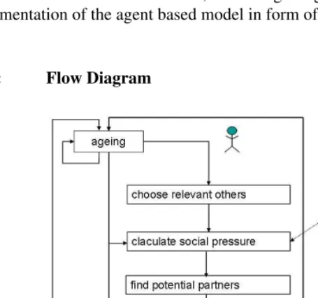
100. Agents who reach the marriageable age of 16start searching for relevant others. The share of married couples among the network of relevant others determines the social pressure function, which then determines together with the age of the agent the region in which unmarried adult agents look for potential partners. In case an agent finds a potential partner, it is checked if the agent herself is among the set of potential partners of his partner. If the latter condition holds, the two agents get married. Figure 6 summarizes the implementation of the agent based model in form of a flow diagram.
Figure 6: Flow Diagram
Married couples give birth to new agents with a probability proportional toasf r(x)
(i.e., the U.S. age specific fertility rate of 1995), in whichxis the age of the bride. Fertility is adjusted to keep the size of the population constant. New born agents are randomly located within an interval which is twice as large as the mothers interval of relevant others.
8Note, that the productsp(pom)∗ai(x)will be between zero and one. By multiplying the product by a
Note, that except year of birth and sex which is randomly chosen assuming a sex ratio at birth of1.048, all other characteristics are missing during childhood. At age 16these characteristics are initialized in a way that is similar to the initial population.
The age–interval to look for relevant others is[x−¯a, x+ ¯a]and we set the length of this interval equal to four years, i.e. ¯a = 2. For the function determining the social pressure we use α = 0.5 and β = 7as the benchmark. For the heterogeneity of the agents with respect to the age interval that determines their network of relevant others we chooseγ¯= 2.
5. Simulation results
We now discuss the results we obtained by running simulations with a population size of
N = 800. We are mainly interested in the hazard of marriage, in order to compare the results obtained from the simulation with macro–level data on age–at–marriage. Since the population contains only800agents, the observed hazard functions exhibit rather erratic patterns. In order to smooth the hazard, we collect the data of75consecutive cohorts and take the average hazard of100simulation runs.
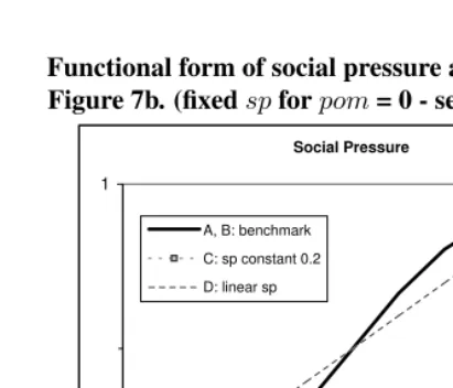
Applying the benchmark setting for the parameters and postulating that the acceptable range for potential partners is only determined by the social pressure and independent of the age of the agent, we obtain the hazard function shown in case A of Figure 7a and Figure 7b for women and men respectively. The fact that hazard of marriage peaks imme-diately at very young ages and then decreases almost monotonically is in contrast to the typical right–skewed bell–shaped distribution observed in empirical data (cf. Figure 1.) Todd et al. (2005) showed that one may obtain a closer fit to the empirical hazard function by introducing heterogeneity among agents (in their case, heterogeneity in the length of adolescents that regulates the beginning of mate search). In our model it is possible to propose an alternative mechanism that is closer to empirical results on social interaction. As discussed in Section 3, network size varies over the life course. Including the age de-pendency of the network size to determine (through social pressure) the acceptable range of potential partners, results in the emergence of a hazard that is qualitatively similar to the one that is well–known (case B, in Figure 7a and Figure 7b).9
To demonstrate that social pressure is a necessary mechanism (in addition to the age influence on the network size) we run further simulations, in which we keep social pres-sure constant for the whole age interval (case C). (Figure 8 plots all alternative functional forms of the social pressure that are applied in the simulations.) Assuming a constant level of social influence results in a steep increase in the marriage hazard function that falls off
9The fact that the hazard rates are lower for men compared to women can be explained by the fact that the
strongly at middle ages. At higher ages almost no one will marry although the age in-fluence on the acceptable range of potential partners is highest for middle–aged agents. Compared to case B, for which social pressure increases with age since more people will be married among the relevant others, case C ignores the increase in social pressure with age.
Figure 7: Hazard of marriage in a population of simulated agents with alternative settings for social pressure. a)Women b)Men
a)
-0.05 0 0.05 0.1 0.15 0.2 0.25
15 25 35 45 55 65 75 85 95
A: ai constant 0.9
B: benchmark
C: sp constant: 0.2
D: linear sp
b)
-0.05 0 0.05 0.1 0.15 0.2 0.25
15 25 35 45 55 65 75 85 95
A: ai constant 0.9
B: benchmark
C: sp constant: 0.2
Further, we show that the choice of an s-shaped function is crucial by simulating the model in the case that social pressure increases linearly (case D). In this case, the hazard of marriage at younger ages is higher due to the higher social pressure at lower marriage proportions and the decay is steeper due to the lower social pressure at higher proportions. There are hardly any marriages above age40(case D).
Figure 8: Functional form of social pressure applied in Figure 7a and Figure 7b. (fixedspforpom= 0 - see Section 4)
Social Pressure
0 1
0 0.1 0.2 0.3 0.4 0.5 0.6 0.7 0.8 0.9 1
pom A, B: benchmark C: sp constant 0.2 D: linear sp
6. Sensitivity analysis
In this section we test the sensitivity of our results when different key parameters are varied. Since the share of married agents among relevant others (pom) within different age–groups plays a key role in determining the age–specific hazard of marriage, we com-pare this share across the alternative parameter settings.
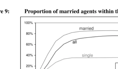
Figure 9 plots the share of married agents within the set of relevant others for single, married and all agents applying the benchmark parameter settings of case B in Figure 7. The low proportion of married relevant others for single agents indicates that agents stay single when they are situated in a group of singles, whereas agents who get married asso-ciate themselves with couples.
Figure 9: Proportion of married agents within the network of relevant others single married all 0% 20% 40% 60% 80% 100% 15-2 0 20-2 5 25-3 0 35-4 0 40-4 5 45-5 0 55-6 0 60-6 5 65-7 0 70-7 5 75-8 0 80-8 5 85-9 0 90-9 5 95-1 00 pom single married all
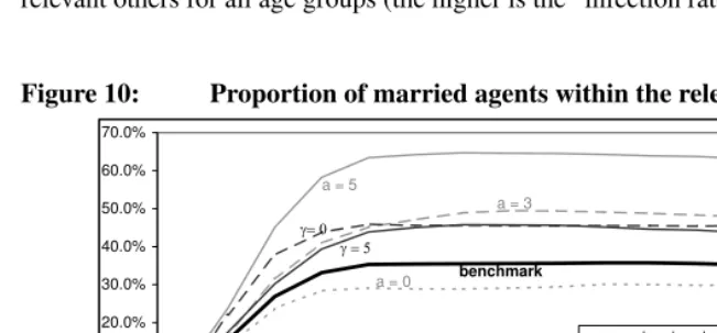
case B in Figure 7 as our benchmark, i.e. we assume a social pressure function that in-creases with age and allow for variations in the network size over age. The benchmark parameter setting isα= 0.5,β = 7,¯a = 2,γ¯ = 2. In comparison to the benchmark settings, we alternatively choose¯γ = 0and¯γ = 5, i.e. we exclude any asymmetry and alternatively increase the asymmetry of the age interval that contains relevant others. Our results indicate for both scenarios higher proportions of married agents among the set of relevant others compared to the benchmark scenario. In case of no asymmetry we see a steep increase at young ages. Due to the symmetry most agents marry at nearly the same (young) age. These early marriages lead to a higher level ofpomat all ages as the willingness to marry spreads. An increase in the asymmetry (¯γ= 5) implies an increase in the variance of the age groups of agents in the set of relevant others. Some agents are only influenced by much older agents, leading to early marriage. Other agents are influ-enced only by much younger agents, which allows marriage at higher ages (because social pressure increase at higher ages). Hence, compared to the benchmark, the proportion of married agents within the set of relevant others is higher at younger ages and compared to the former scenario (γ¯= 0) it increases for a longer period. For both scenarios (¯γ= 5
and¯γ= 0) the hazard of marriage will be above the benchmark case at all ages.
implies an increase in the proportion of married agents. The wider the interval the more likely young agents are influenced by older agents who are more likely to be married. The more agents marry at young ages the higher becomes the share of married agents among relevant others for all age groups (the higher is the “infection rate”).
Figure 10: Proportion of married agents within the relevant others
benchmark
a = 0
a = 3 a = 5
J J 0.0% 10.0% 20.0% 30.0% 40.0% 50.0% 60.0% 70.0% 15-2 0 20-2 5 25-3 0 35-4 0 40-4 5 45-5 0 55-6 0 60-6 5 65-7 0 70-7 5 75-8 0 80-8 5 85-9 0 90-9 5 95-1 00 pom
benchmark a = 0
a = 3 a = 5
J J
To test the sensitivity of our results with respect to changes in the functional form of the social pressure function we run simulations in which we change alternatively the inflection point and the slope of the social pressure function. The alternative set of exper-iments is summarized in Figure 11a and Figure 11b for women and men. The alternative forms of the social pressure function are plotted in Figure 12. As the benchmark settings of our simulations we choose again case B in Figure 7 (i.e. β = 7, α = 0.5). Our re-sults indicate that if the inflection point of the social pressure function shifts to the left (α = 0.45), i.e. social pressure increases at each age, the resulting hazard increases mostly at younger ages. A change in the slope of the social pressure function keeping the inflection point the same (β = 8) implies a reduction in the hazard. Due to social in-fluence, lower marriage hazards at younger ages obviously translate into lower marriage hazards at higher ages as well.
7. Summary and discussion
Figure 11: Hazard functions for marriage in a population of simulated agents with alternative settings for social pressure. a) Women b) Men
a)
-0.05 0 0.05 0.1 0.15 0.2 0.25
15 25 35 45 55 65 75 85 95
E D E D E D
b)
-0.05 0 0.05 0.1 0.15 0.2 0.25
15 25 35 45 55 65 75 85 95
Figure 12: Functional form of social pressure applied in Figure 11a and Figure 11b.
Social Pressure
0 1
0 0.1 0.2 0.3 0.4 0.5 0.6 0.7 0.8 0.9 1 pom
E D E D E D
that intervene between social structure and marriage patterns according to Dixon (1971):
availabilityof mates anddesirabilityof marriage. In our population of agents, the avail-ability of mates is modeled by considering the set of potential partners, in particular also by the age–dependent network size, and by the method of selection (two–sided search). The desirability of marriage is modeled by considering explicitly the dynamics of social pressure.
The results of our simulations show that the agent–based model we propose can re-produce the shape of the hazard of marriage that is typically observed at the population level. In other words, the hazard functionemergesfrom the bottom–up in our model. The model we present includes a set of parameters that need to be calibrated with actual data. However, our numerical simulations indicate that the qualitative form of the hazard is rather robust towards changes in parameters that determine the size of the set of relevant others as well as the slope of the social pressure function.
Through an additional set of numerical simulations, we investigated the sensitivity of our results with respect to the parameters that determine a) the size of the network of relevant others or b) the strength of social pressure by agents who are already married in the network of relevant others. These parameters have a pronounced effect on the share of married people in the network of relevant others and on the propensity to get married in general. An empirical validation of those parameters for different societies constitutes an additional avenue for further research.
References
[1] Aparicio Diaz, B., Fent, T. (2006). An Agent–Based Simulation Model of Age– at–Marriage Norms. In: Billari, F. C., Fent, T., Prskawetz, A., Scheffran, J. (eds.) Agent–Based Computational Modelling. Heidelberg: Physica Verlag, pp. 85–116. [2] Bernardi, L. (2003). Channels of social influence on reproduction, Population
Re-search and Policy Review, 22(5-6), pp. 527-555.
[3] Billari, F.C. (2001). A log-logistic regression model for a transition rate with a start-ing threshold. Population Studies, 55(1), pp. 15–24.
[4] Billari, F.C., Prskawetz, A. (eds.) (2003). Agent–Based Computational Demogra-phy: Using Simulation to Improve our Understanding of Demographic Behaviour. Heidelberg: Physica Verlag.
[5] Billari, F.C., Prskawetz, A., Fürnkranz, J. (2003). On the Cultural Evolution of Age–at–Marriage Norms. In: Billari, F.C. and Prskawetz, A. (eds.) Agent–Based Computational Demography: Using Simulation to Improve our Understanding of Demographic Behaviour. Heidelberg: Physica Verlag, pp. 139–157.
[6] Bongaarts, J., Watkins, S.C. (1996). Social Interactions and Contemporary Fertility Transitions, Population and Development Review 22(3), pp. 639–682.
[7] Clark, A.E., Oswald, A.J. (2002). Well-Being in Panels. Paris: CNRS and Delta. [8] Coale, A.J. (1971). Age Patterns of Marriage, Population Studies, 25, pp. 193–214. [9] Coale, A.J., McNeil, D.R. (1972). The Distribution by Age of the Frequency of First Marriage in a Female Cohort, Journal of the American Statistical Association, 67, pp. 743–749.
[10] Coltrane, S.L., Collins, R. (2001). Sociology of Marriage and the Family-Gender, Love, and Property. 5th ed. Belmont, CA: Wadsworth.
[11] Dixon, R.B. (1971) Explaining cross-cultural variations in age at marriage and pro-portions never marrying, Population Studies 25, pp. 215–233.
[12] Due, P., Holstein, B., Lund, R., Modvig, J., Avlund, K. (1999). Social relations: network, support and relational strain. Social Science & Medicine 48(5), pp. 661-673.
[13] Hammer, M., Gutwirth, L., Phillips, S. L. (1982). Parenthood and Social Networks: A preliminary view. Social Science & Medicine, 16(24), pp. 2091–2100.
[14] Hernes, G. (1972). The process of entry into first marriage. American Sociological Review, 37, pp. 47–82.
[15] Kalick, S.M., Hamilton, T.E. (1986). The Matching Hypothesis Reexamined. Jour-nal of PersoJour-nality and Social Psychology, 51, pp. 73–82.
[16] Kalmijn, M. (1998). Intermarriage and Homogamy: Causes, Patterns, Trends. An-nual Review of Sociology, 24, pp. 395–421.
Gen-eralized Log Gamma Distribution A New Identity and Empirical Enhancements. Demographic Research, 9(10).
[18] Kohler, H.P., Behrman, J.R., Skytthe, A. (2005). Partner + Children = Happiness? The Effect of Fertility and Partnerships on Subjective Well–Being. Population and Development Review, 31(3), pp. 407–445.
[19] Marsden, P.V. (1987). Core Discussion Networks of Americans. American Socio-logical Review, 52, pp. 122–131.
[20] Micheli, G.A. (2000). Kinship, Family and Social Network: The anthropological embedment of fertility change in Southern Europe. Demographic Research 3, 13. [21] Montgomery, M.R., Casterline, J. (1996). Social Influence, Social Learning, and
New Models of Fertility. In: Casterline, J., Lee, R., Foote, K. (eds.) Fertility in the United States: New Patterns, New Theories. Supplement to Population and Devel-opment Review, 22(1): pp. 151-175.
[22] Montgomery, M.R., Casterline, J. (1998). Social networks and the diffusion of fertil-ity control. Policy Research Division Working Paper No. 119. New York: Population Council.
[23] Morgan, D. L. (1988). Age Differences in Social Network Participation. Journal of Gerontology 43(4), pp. 129–37.
[24] Nazio, T., Blossfeld, H.-P. (2003). The Diffusion of Cohabitation among Young Women in West Germany, East Germany and Italy. European Journal of Population 19, pp. 47-82.
[25] Simão, J., Todd, P.M. (2003). Emergent patterns of mate choice in human popula-tions. Artificial Life 9, pp. 403-417.
[26] van Tilburg, T. G. (1995). Delineation of the social network and differences in net-work size. In: Knipscheer, C. P. M., de Jon Gierveld, J., Tilburg, T. G., Dykstra, P. A., eds. Living Arrangements and Social Networks of Older Adults. Amsterdam: VU University Press.
[27] van Tilburg, T. G. (1998). Losing and gaining in old age: changes in personal net-work size and social support in a four–year long study. Journals of Gerontology Series B, 53(6), pp. 313–323.
[28] Todd, P. M., Billari, F. C. (2003). Population–Wide Marriage Patterns Produced by Individual Mate–Search Heuristics. In: Billari, F. C., Prskawetz, A. (eds.), Agent– Based Computational Demography: Using Simulation to Improve our Understand-ing of Demographic Behaviour. Heidelberg: Physica Verlag, pp. 117-137.
[29] Todd, P. M., Billari, F. C., Simão, J. (2005). Aggregate Age–at–marriage Patterns from Individual Mate Search Heuristics. Demography 42(3), pp. 559–574.
[31] Wagner, M., Wolf, C. (2001). Altern, Familie und soziales Netzwerk. Zeitschrift für Erziehungswissenschaft 4, pp. 529–554.