Test Plan for Real-Time Modeling & Simulation of Single Pole Switching Relays

(1)

University of New Orleans University of New Orleans

ScholarWorks@UNO

University of New Orleans Theses and

Dissertations Dissertations and Theses

Spring 5-13-2016

Test Plan for Real-Time Modeling & Simulation of Single Pole

Switching Relays

Ram Mohan Sanaboyina

University of New Orleans, New Orleans, [email protected]

Follow this and additional works at: https://scholarworks.uno.edu/td

Part of the Electrical and Electronics Commons, and the Power and Energy Commons

Recommended Citation Recommended Citation

Sanaboyina, Ram Mohan, "Test Plan for Real-Time Modeling & Simulation of Single Pole Switching Relays" (2016). University of New Orleans Theses and Dissertations. 2215.

https://scholarworks.uno.edu/td/2215

This Thesis is protected by copyright and/or related rights. It has been brought to you by ScholarWorks@UNO with permission from the rights-holder(s). You are free to use this Thesis in any way that is permitted by the copyright and related rights legislation that applies to your use. For other uses you need to obtain permission from the rights-holder(s) directly, unless additional rights are indicated by a Creative Commons license in the record and/or on the work itself.

This Thesis has been accepted for inclusion in University of New Orleans Theses and Dissertations by an

(2)

Test Plan for Real-Time Modeling & Simulation of Single Pole Switching Relays

A Thesis

Submitted to Graduate Faculty of the University Of New Orleans

in partial fulfilment of the requirements for the degree of

Master of Science In

Engineering Electrical Engineering

By

Ram Mohan Sanaboyina

B.Tech. JNTU, 2006

(3)

Acknowledgement

Firstly, I would like to express my utmost gratitude to my adviser Dr. Ittiphong Leevongwat for his

full support, encouragement and always making his time available for suggestions and comments.

This thesis would not have been possible without his guidance and help who in one way or another

contributed and extended his valuable assistance in the preparation and completion of this study.

I am also grateful to Professor Dr. Parviz Rastgoufard for his valuable suggestions,

technical support and guidance in the right direction throughout my thesis, academic research and

course work during my master studies.

I would like to thank Dr. Ebrahim Amiri for taking time out from his busy schedule to

serve as a member of my committee.

I would also like to thank Rastin Rastgoufard for his help in acquiring technical and

software knowledge required for completing the tasks in this thesis.

I sincerely thank Mark Allen from Entergy Services, Inc. for his time and valuable

guidance in developing part of this work.

I would also like to acknowledge the support from OPAL-RT personnel in helping with

”HYPERSIM” modeling while conducting this research work.

Finally, I would like to acknowledge and thank my parents, my wife, my brothers and

(4)

List of Figures

2.1 Distributed Transmission Line [1] . . . 13

2.2 Equivalent circuit of One Mode of a Transmission Line [2] . . . 15

2.3 Equivalent Circuit of Three-Winding Transformer [3] . . . 16

2.4 Equivalent Circuit for Three-Phase Induction Motor [4] . . . 18

2.5 No-Load Test Equivalent Circuit-1 for Three-Phase Induction Motor [4] . . . 18

2.6 No-Load Test Equivalent circuit-2 for Three-Phase Induction Motor [4] . . . 19

2.7 Locked-Rotor Test Equivalent Circuit for Three-Phase Induction Motor [4] . . . 20

2.8 Simplified Equivalent Circuit for Three-Phase Induction Motor Under Load [4] . . . 20

2.9 Inductor Branch [2] . . . 24

2.10 Equivalents of Inductor Branch using the Trapezoidal Rule [2] . . . 24

2.11 Capacitor Branch [2] . . . 25

2.12 Equivalent of Capacitor Branch using the Trapezoidal Rule [2] . . . 26

3.1 Methodology . . . 30

3.2 Work Flow . . . 32

3.3 T-Line Geometry . . . 34

3.4 Python Output of Transmission Line of Figure 3.3 . . . 35

3.5 Control Panel of an Untransposed Line . . . 36

3.6 Control Panel of a J-Marti Line . . . 37

3.7 Control Panel of an Induction Motor . . . 39

3.8 Control Panel of a Two-Winding Transformer . . . 40

3.9 Control Panel of a Three Winding Transformer . . . 42

3.10 Sensitivity Analysis FLowchart . . . 44

3.11 Primary Arc Block Diagram . . . 45

3.12 Secondary Arc Block Diagram . . . 46

3.13 User Code Module Simulation Flowchart . . . 47

3.14 Switch Simulation Flowchart . . . 48

3.15 Relay Topology . . . 50

3.16 Relay Test Setup . . . 51

4.1 Test System . . . 55

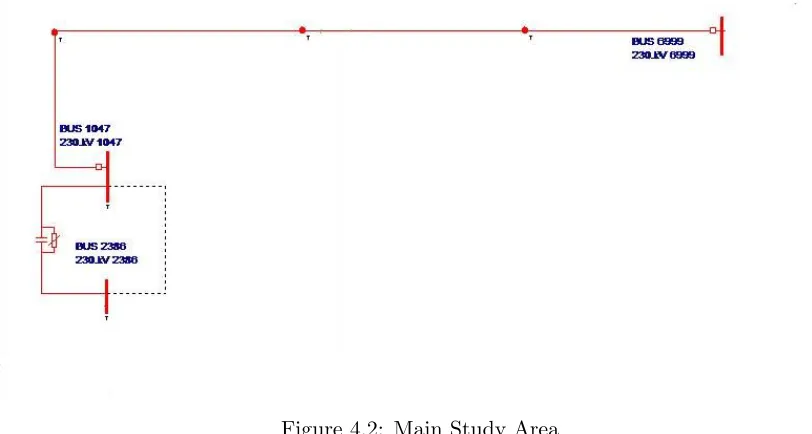
4.2 Main Study Area . . . 56

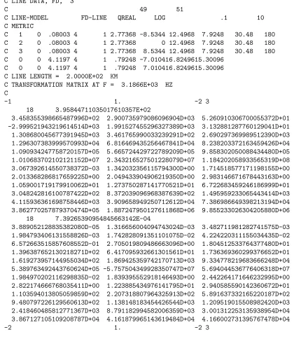
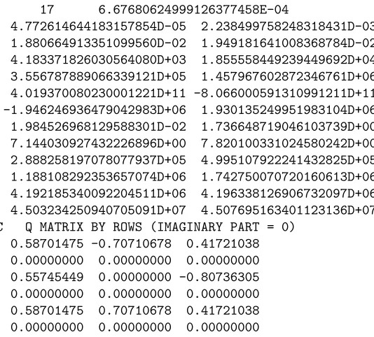
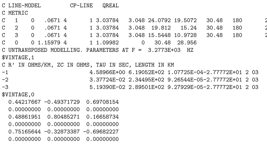
4.3 Punchfile of Transmission Line Section BUS-1047 - BUS-6999 Part 1 . . . 58

4.6 Punchfile of Transmission Line Section BUS-1054 - BUS-1733 . . . 60

(7)

4.15 EMTP Punch file for BC-Tran Three Winding Transformer At Bus-1071 . . . 69

4.16 EMTP Punch file for BC-Tran Three Winding Transformer At Bus-2387 . . . 70

4.17 Control Panel of Series Capacitor . . . 72

4.18 Control Panel of Surge Arrester . . . 73

4.19 Control Panel of Shunt Capacitor . . . 74

4.20 Control Panel ofπ Line . . . 77

5.1 Model of IPO System . . . 79

5.2 Series Capacitor Line . . . 80

5.3 Local End Breaker Arrangement . . . 81

5.4 Remote End Breaker Arrangement . . . 81

5.5 Series Capacitor Protection Arrangement . . . 82

5.6 Fault & Line Currents for Phase A to Ground Faults at Local End . . . 84

5.7 Voltages at Terminal Buses for Phase A to Ground Faults at Local End . . . 85

5.8 Fault & Line Currents for Phase A to Ground Faults at Mid-Line . . . 87

5.9 Voltages at Terminal Buses for Phase A to Ground Faults at Mid-Line . . . 88

5.10 Fault & Line Currents for Phase A to Ground Faults at Remote End . . . 90

5.11 Voltages at Terminal Buses for Phase A to Ground Faults at Remote End . . . 91

5.12 Fault Arc Model . . . 93

5.13 Primary Arc Block Diagram . . . 93

5.14 Secondary Arc Block Diagram . . . 94

5.15 Fault Arc Model Test System . . . 95

5.16 Primary Arc Plots . . . 96

5.17 Primary Arc Resistance . . . 96

5.18 Primary Arc Voltage . . . 97

5.19 Secondary Arc Plots . . . 98

5.20 Secondary Arc Current . . . 98

5.21 Secondary Arc Voltage . . . 99

5.22 Switch Simulation . . . 99

5.23 Line 1 Relay Inputs from HYPERSIM . . . 100

5.24 Line 2 Relay Inputs from HYPERSIM . . . 101

5.25 Line 1 Relay Outputs to HYPERSIM . . . 102

5.26 Line 2 Relay Outputs to HYPERSIM . . . 103

5.27 Line 1 Brekaer Close and Fail Circuit . . . 104

(8)

List of Tables

1.1 Application Requirements for Relay Testing [7] . . . 3

1.2 Relative Number of Different Types of Faults on HV transmission lines [8] . . . 6

1.3 Relative Number of Different Types of Faults on 525 kV transmission lines [8] . . . . 6

4.1 π Line Data . . . 57

4.2 Voltage Sources Data . . . 66

4.3 Two-Winding Transformer Data . . . 66

4.4 Two-Winding Transformer Data (HYPERSIM) . . . 67

4.5 Bus 1071 & Bus 2387 Three-Winding Transformer Excitation Data . . . 68

4.6 Bus 1071 & Bus 2387 Three-Winding Transformer Positive & Zero Sequence Data . 68 4.7 Bus 1071 Three-Winding Transformer Winding Data . . . 68

4.8 Bus 2387 Three-Winding Transformer Winding Data . . . 68

4.9 Bus 1071 Three-Winding Transformer Short Circuit Data . . . 68

4.10 Bus 2387 Three-Winding Transformer Short Circuit Data . . . 68

4.11 Induction Motor General Data . . . 71

4.12 Induction Motor Performance Data . . . 71

4.13 Induction Motor Data (HYPERSIM) . . . 71

4.14 Power Transformer Data . . . 72

4.15 Power Transformer Data (HYPERSIM) . . . 72

4.16 Series Capacitor Data (HYPERSIM) . . . 72

4.17 Surge Arrester Data (HYPERSIM) . . . 73

4.18 Shunt Capacitor Data (HYPERSIM) . . . 74

4.19 Equivalent Voltage Sources Data . . . 75

4.20 Two-Winding Equivalent Transformer Data . . . 76

4.21 Two-Winding Equivalent Transformer Data (HYPERSIM) . . . 76

4.22 Equivalentπ Lines Data . . . 77

5.1 Maximum Phase A to Ground Fault Currents (A) for Local End Fault (1 ∼25) . . . 83

5.2 Maximum Phase A to Ground Fault Currents (A) for Local End Fault (26 ∼50) . . 83

5.3 Maximum Phase A to Ground Fault Currents (A) for Mid-Line Fault (1∼ 25) . . . 86

(9)

Abstract

A real-time simulator (RTS) with digital and analog input/output modules is used to conduct

hardware-in-the-loop simulations to evaluate performance of power system equipment such as

pro-tective relays by exposing the equipment to the simulated realistic operating conditions. This work

investigates the use of RTS to test relays with single-pole-switching (SPS) feature. Single-pole

switching can cause misoperations due to fault arc during reclosing of the breakers. Through this

investigation, a test procedure appropriate for the testing SPS relays has been developed. The

test procedure includes power system modeling for real time simulation, relay test setup, and test

plan. HYPERSIM real-time simulator was used to model an actual power system.

Transmis-sion lines, three-winding transformers, and induction motor were modeled with actual parameters.

Models for fault arc in HYPERSIM real time simulator were developed. Test set-up for evaluating

relay performance and wiring drawings for connecting relay in closed-loop to the simulator were

developed.

(10)

Chapter 1

Introduction

This chapter summarizes the background of this work and presents a literature review on protective

relay testing using real-time modeling and simulation. The chapter concludes with the scope of

work for the thesis.

1.1 Overview of Real Time Digital Simulators

“Real time digital simulator (RTS) applied for power systems provide power systems simulation

technology for fast, reliable, accurate and cost-effective study of power systems. The RTS is a full

digital electromagnetic transient power system simulator operates in real time, tests physical devices

and performs studies quickly” [9]. In RTS, computer models of the power system are simulated in

real-time to analyze the hardware-in-the-loop performance of the power system components under

more realistic conditions [10]. The following are the major applications of RTS mentioned in [11].

• Specification study

(11)

• Protective relays and power semiconductor equipments (HVDC and FACTS devices)

pre-commissioning and performance analysis.

[10] The benefit of performing hardware-in-the-loop simulations of power system

equip-ment is increased efficiency in the conduct of the tests and it is required for evaluating the

perfor-mance of the equipment. The following are the situations where hardware-in-the-loop simulation

is required.

1. Relays in fast re-closing & single pole auto-reclose of transmission lines.

2. Relays for out-of-step protections & distribution feeders with reclosure.

3. Relays responding to frequency excursions.

4. Power system stabilizers for excitation control system of generators.

5. Special breaker controllers.

[10] Dynamics caused in the power system due to tripping and re-close actions of relays

can be captured and analyzed by hardware-in-the-loop testing of relays. Hardware-in-the-loop

simulation of stabilizer determines its effectiveness on power system stability and simulations for

controlled opening and closing of individual breaker poles are advantageous in reactor switching

and capacitor switching respectively.

1.1.1 History of Real-Time Simulator

The early RTS [7] used digital technology utilizing power system and fault modeling capabilities of

electromagnetic transient programs to implement protective relay testing simulators. This approach

is flexible to the user to model the system accurately. These simulators are advantageous in meeting

(12)

the relay and the simulator. In the later years, a new real-time simulator was developed for real

time testing of protection relay to evaluate relay’s performance and also to determine which relay

suites best for a given application. Table 1.1 [7] summarizes application requirements that the

simulator design required to meet for testing relays.

Table 1.1: Application Requirements for Relay Testing [7]

Applications Requirements

Parallel Lines Three terminal simulator configuration and coupled RL branches modeling

Series compensated long lines Modeling of distributed and frequncy dependent parameter lines

MOV and arrester protection Modeling for short line representation

Close-in and Far-end faults PI circuit modeling for short line representation

Single-pole auto reclosing Real-time interaction, modeling of circuit breakers and switches

Different fault cases Selection of fault type, resistace, incidence angle and location

Influence of relaying transformers Accurate modeling of CCVT and CT transient response

Timing sequence of circuit breakers Modeling of circuit breaker timing logic

The following are the commercially available RTS in today’s market [9]:

• RTDS developed by RTDS technologies Inc.

• HYPERSIM developed by Hydro-Quebec.

• eMEGAsim developed by OPAL-RT Technologies Inc.

1.2 A Review of Real Time Digital Simulator for Relay Testing

Many research papers [10]-[12], published on testing relays using RTS, evaluating the performance

of relays and determining best protection principles. A numerical distance relay incorporated with

new positive sequence directional element was tested with RTDS for verifying the operation of

directional element incorporated in the relay in [13]. In [14], Numerical Distance relay performance

(13)

the RTDS. The results of these digital simulations are compared with dynamic simulation results

for validation of high performance relays. Line protection relays and transformer protection relays

were tested and evaluated using the RTS,AREN ET M for fault cases applied on the protected line

between the two series capacitor banks in [15]. In [10], Test setup for hardware-in-the-loop testing

of a feeder relay, a power system stabilizer, and a circuit breaker controller were described. In [16],

tests on the existing line relays were carried out to obtain settings for the relays for all the possible

operating conditions and to determine deficiency in the performance of the relay.

The work published in [17] compared the performance of different line protection systems

on Hydro-Quebec series compensated network to determine the best protection principles. A

dis-tance relay and a PCM current differential relay tested using the RTDS for verifying the scenarios in

which relay fails to operate as desired in [18]. Relay configured for over-current scenario was tested

and analyzed for closed loop performance using RTDS in [19]. In this publication, effect of CT

sat-uration on closed loop performance of relays was also analyzed. Performance of Numerical Distance

Relay using RTDS was evaluated in paper [20]. Different scenarios including fault types, positions,

inception angles and fault resistances were used for evaluating relay transient performance. An

actual relay was tested using automatic testing procedure and manual testing procedure in [21].

This publication identified which approach is best suited for testing and analyzing the performance

of relays for a particular fault scenario of interest.

M. Kezunovicl and M. McKenna in [7] tested RTS for accuracy of producing and speed

of calculating fault transients. A full and reduced models of series capacitor power system network

were developed. A single phase to ground fault was applied and the relay was tested for accuracy

and speed for both the models. EMTP and RTS waveforms were compared for the same fault event

to determine the accuracy of simulation. Time step required to carry out simulations in real-time

(14)

Most of the relays tested with RTS use lumped parameter line models for transmission

lines in the power system networks. In publications [7] and [17], distributed frequency dependent

line model was used for transmission lines in the power system network. In papers [7], [17], [13] and

[15], the test system modeled and simulated for testing relays includes a series capacitor. Effect of

CT and CVT on the performance of relays was analyzed in [14] and [20]. Load was modeled as

constant impedance and motor load in [17] and as an inductive motor load in [14]. In majority of

the research publications, sources were modeled as constant voltage sources behind impedance’s.

In [14], source was modeled as generator. Effect of shunt compensation on the performance of

relays was analyzed in papers [17], [13] and [14]. In [17], power system network used for studying

the performance of line protection system consists of equivalents for voltage levels below 315kV.

Network simulation in [17], include transformer saturation and the power system network in [13]

has three-winding transformer model.

1.3 Overview of Single Pole Switching

Single pole switching (SPS), which is a combination of single-pole tripping (SPT) and single-pole

reclosing (SPR) is a feasible approach to the operation of power systems. According to [22], SPS

application on transmission lines is a useful and feasible means to improve power system reliability.

In [23] SPT is defined as “Opening of faulted phase due to single line to ground fault” and SPR

as “re-closing of the faulted phase following a single pole trip”. SPS applications on transmission

line open a single pole of the transmission line breakers in the event of fault keeping the other two

poles intact. The two ends of the transmission line are metallically connected via other two poles

allowing transfer of power and reduce the possibility of loosing synchronism [24]. SPS application

improves power system stability and in [25] it was shown that the stability is maintained due to

(15)

machines. In [26], it was shown that SPS application on transmission lines for all temporary

single-line-to-ground faults, automatic generator shedding and automatic load shedding conditions were

prevented and voltage stability margins were also improved during single pole open period due to

flow of smaller amount of reactive power from the system.

Majority of faults occurring on HV transmission lines are single line to ground faults,

SPAR takes advantage of this fact. Table 1.2 [8] shows the statistics of percent of different types

of faults occur on HV transmission lines.

Table 1.2: Relative Number of Different Types of Faults on HV transmission lines [8]

Fault type Percent

LG 70

LL 15

LLG 10

3L 5

Total 100

The spacing between conductors on EHV/UHV lines is more, therefore the percentage

of multi-phase faults is less. Table 1.3 [8] shows the statistics of percent of different types of faults

that occur on a 525 kV transmission lines.

Table 1.3: Relative Number of Different Types of Faults on 525 kV transmission lines [8]

Fault type Percent

LG 93

LL 4

LLG 2

3L 1

(16)

The following are the benefits of SPS application on transmission lines listed in [23]:

• Transient state stability improvement.

• System reliability improvement and availability of system with one or two transmission lines.

• Switching over voltages reduction.

• Shaft torsion oscillations reduction.

In spite of benefits associated with SPS schemes [26], some utilities still do not apply this technology

for the following reasons:

• Additional expense for breakers.

• Added complexity in the protection scheme.

• Presence of secondary arc.

• Added stress to the generating units.

The dynamic interaction between a fault arc and the power system is extremely

impor-tant to determine the insimpor-tant of successful reclosure of a faulted system [5]. The success of SPS

application depends on a number of parameters such as secondary arc current, recovery voltage

across the arc path, arc location and meteorological conditions.

[26] A single line to ground fault results in the formation of primary arc between the

faulted phase and ground. The fault is isolated by the line protection system by tripping the single

pole of the breaker in SPS applications, there by extinguishing the primary arc. The two ends of

the transmission line are metallically connected by the other two healthy phases during the single

pole open period. Voltage is induced in the open phase conductor due to capacitive and inductive

coupling between the healthy phase conductors and open phase conductor. As the air is already

(17)

For successful reclosure, it is essential to detect extinction of secondary arc. In case of

500kV lines, special compensation schemes become necessary to limit the secondary arc current and

recovery voltage to ensure successful high speed re-closing. The published literature [27] says that

the behavior of secondary arc current can be studied through simulation or by means of recording

naturally occurring or staged faults. Naturally occurring faults are unpredictable and staged fault

tests are expensive and complex to perform. Real time simulation with a RTS can overcome many

of these problems.

1.4 A Review on Single Pole Switching Studies

Research on single pole switching focuses on advantages of having SPS schemes, challenges with

SPS applications. [8], [22], and [27] - [28] presented findings on SPS applications on power systems.

According to published literature [29] majority of faults occurring on a 132kV line were

single phase to ground faults and successful single pole tripping and re-closing was recorded for

most of the cases. Also [29] discusses the advantages of having single pole tripping over multi-pole

tripping in that better system stability and minimization of overall system disturbances during fault

clearing operations. In [30] Reactor compensation makes the extinction of secondary arc possible by

reducing the phase to ground fault current in the open phase of the line. The degree of compensation

required to limit the secondary arc current to a level that can be extinguished depends on the length

of the line. Greater the length of the line greater the degree of compensation. Affects of shunt

reactor compensation on successful reclosure, secondary arc extinction and stability of the power

system during SPS operation on 500 kV system were verified by conducting staged fault tests in

[31]. Transient stability limit and critical clearing time are compared for single pole switching and

three pole switching in paper [32]. The problems with implementing single pole switching (SPS)

(18)

one pole of circuit breakers at both ends of a transmission line for clearing single line to ground

fault produces high negative sequence current in nearby generators.

Single pole opening induces voltage across secondary arc path after the extinction of

primary arc. The induced voltage is called as Recovery Voltage. [35] [36] [37] discuss this recovery

voltage. In [35], the transient recovery voltages of a transposed transmission system with neutral

reactor and un-transposed system during single-pole switching operation were compared. In [36],

maximum possible transient recovery voltage for a transmission system during SPS operation was

determined by varying fault application time, position and duration of faults. In [37], it was shown

that magnitude of secondary arc current and recovery voltage determines the success of re-close

operation on 765 kV system. [38] and [39] discuss the methods to minimize the secondary arc

current.

In [27],[40],[41],[42] and [43], modeling and simulation of primary and secondary arc using

various modeling softwares were published. Realistic arc models were developed and incorporated

in EMTP in [42] based on mathematical models developed by A.T. Johns, R.K. Aggarwal and

Y.H. Song [40]. [42] investigated single phase re-closing using arc model on single and double

circuit transmission line to determine the characteristics of secondary arc current for single phase

to ground faults. Realistic arc models are developed using FORTRAN statements and incorporated

in ATPDraw in [43] based on mathematical models developed by M. Kizilcay, G. Ban, I. Prikler, P.

Handl [41]. [43] validated primary and secondary arc models and implemented on a power system

to verify the settings for SPAR protection scheme. Arc models developed and simulated in real

time in [27] to determine the response of relays with secondary arc detection and to identify the

(19)

1.5 Scope of Work

The work done in this thesis is continuation of work published in [12] and [44]. [12] focused on

evaluating performance of various digital line protection relays using a closed-loop real-time power

system digital simulator called ””HYPERSIM”” to determine the best suited protection scheme

for a series capacitor line. An equivalent test system was modeled in HYPERSIM and distance

relays of two different manufacturers and a differential relay were connected in closed loop with the

real-time simulator at each end of the line. Different fault scenarios were performed and relays were

tested to verify their expected performance. Distance relays were found to have deficiencies and

differential relay successfully cleared all internal faults. The test results concluded that for series

capacitor lines dual primary differential relays with back up distance and over-current elements

to be used with Zone 1 distance elements turned off. The study continued in [44] by replacing

the existing relays with two dual primary differential relays in loop with the real-time simulator

and tested with the same scenarios for evaluating the performance of these new relays. The tests

performed on the system concluded that the relays did not operate as intended in a few scenarios.

This thesis is part of an investigation of Single Pole Switching (SPS) in commercial

protective relays used in electrical system protection scheme. The main objective of this work is

to create a test plan to evaluate the performance of two different digital line differential protection

relays that are configured to control IPO breakers modeled in real-time simulator. The second

objective of this work is to design a test setup, including necessary signals appropriate for capturing

the performance of SPS operation.

The following tasks were performed to achieve the two objectives:

• A portion of a power system which is two-bus deep from the protected series capacitor line

(20)

comprises of the study area with detailed parameters for accurate line models, motor load

models, two-winding and three-winding transformer models, series capacitor with surge

ar-rester and shunt capacitor components. The rest of the power network is equivalenced in

ASPEN to voltage sources, transformers andπ lines.

• Investigation on implementation of fault arc models in HYPERSIM real time simulator is also

carried out in this thesis. Arc models would help capture the effect of the remaining active

phases when only single phase is tripped in SPS operation.

• Systematic study is performed to select the worst case switch timings for the faults that result in the worst fault currents. The selected faults are performed on a line with series capacitor

connected at one end and high capacity motor connected at the other end. Close-in faults

(close to series capacitor bus), faults at middle of line, and remote faults (close to motor bus)

are applied automatically at different incidence angles for each scenario in order to determine

the worst case switch time.

• Test setup includes the design of line differential relays protection schematics to include breaker trips, breaker status, breaker close and breaker fail logic’s for testing the protection

(21)

Chapter 2

Mathematical Formulation

The previous chapter has already given some idea on relay testing and single pole switching

ap-plications. Reminding once again, the main objective of this work is to come up with a power

system model suitable for testing relays in hardware-in-the-loop for single pole switching

applica-tions. In view of this, this chapter discusses mathematical modeling of power system components

in the model developed in this thesis and background of power system components modeling in

HYPERSIM real time simulator software. Background of mathematical models and HYPERSIM

models of power system components used in this thesis are illustrated in section 2.1 to section 2.4.

2.1 Transmission Lines [1]

A Transmission line is characterized by four distributed parameters: series resistance, series

in-ductance, shunt conin-ductance, and shunt capacitance. Magnetic and electric effects around the

conductor are represented by series inductance and shunt capacitance and leakage current along

insulator strings and ionized pathways in the air is represented by shunt conductance. In this thesis,

transmission lines are modeled as distributed parameter lines. Let us look into the mathematical

(22)

2.1.1 Mathematical Model of Transmission Line

The per phase circuit diagram of a transmission line is shown in Figure 2.1. l be the length of the

transmission line, V1, I1 be the sending end bus voltage and current, V2, I2 be the receiving end

bus voltage and current,z be the series impedance per meter, andy be the shunt admittance per

meter to neutral. z,y are represented by equations Equation 2.1 and Equation 2.2.

z=r+jωl (2.1)

y=g+jωc (2.2)

Figure 2.1: Distributed Transmission Line [1]

The relation between sending end and receiving end of transmission line is represented

by Equation 2.3 and Equation 2.4.

V1 =V2coshγl+ZcI2sinhγl (2.3)

I1 =I2coshγl+

V2

Zc

(23)

where

γ =∆√yz (2.5)

is called the propagation constant.

Rewriting Equation 2.3 and Equation 2.4 as Equation 2.6 and Equation 2.7 respectively.

V1 =AV2+BI2 (2.6)

I1 =CI2+DV2 (2.7)

where

A= coshγl (2.8)

B =Zcsinhγl (2.9)

C = coshγl (2.10)

D= V2

Zc

sinhγl (2.11)

Rearranging Equation 2.6 and Equation 2.7 in matrix form, we get Equation 2.12

    V1 I1     =     A B C D         V2 I2     (2.12) T =     A B C D     (2.13)

(24)

2.1.2 HYPERSIM Model of Transmission Line [2]

The equivalent circuit representing a single mode of a transmission line is shown in Figure 2.2.

2 - 10

Trapezoidal integration

and past currents at both terminals. Equivalent at each terminal can therefore be

calculated in parallel.

Model for frequency dependent lines uses the same philosophy but with a more

complex equivalent.

Each half (left and right) of the line equivalents will be converted from mode to phase

form and incorporated into the corresponding substation equation to be solved with

other elements.

2.3 Substation modelling

In each substation, there are passive components interpreted as RLC elements which

can be linear or non-linear, circuit-breakers, different kinds of generation interpreted

as voltage and current sources equipped with control systems. Machines and motors

are considered as sources with control systems.

Beside control systems, other equipments are power elements working at the power

system level voltages and currents. Power elements of a substation are interconnected

together via nodes. Power elements are not simulated sequentially one by one but

rather simultaneously all together in a single equation call the

node equation

:

(9)

where

Y

is the substation admittance matrix,

V

is vector of node voltages and

I

is

vector of node currents (currents injected to nodes).

Control systems are modeled using the bloc diagram principle, either under graphic

form (Hypersim bloc diagram and Simulink bloc diagram) or coded in C/C++. Their

inputs can be node voltages and currents while their outputs can be used to control

sources and switches.

2.3.1 RLC

ELEMENT

Trapezoidal integration

Hypersim, as EMTP, uses the trapezoidal integration technique, it means that

J_mK _J

mM

Z_c RT 4 ---+ _Z c R_T 4 ---+ I_mK V_mK +

-K

M

V_mM I_mM

+

-Figure 2 : Equivalent circuit of one mode of a transmission line

YV

=

I

Figure 2.2: Equivalent circuit of One Mode of a Transmission Line [2]

A single mode line model is represented at each terminal (sending end and receiving

end) as an equivalent circuit composed of a current source in parallel with a resistor. The current

source at terminal K is given by Equation 2.14.

JmK =

1−h

2

VmK(t−τ)

Req

+hImK(t−τ)

+

1 +h

2

VmM(t−τ)

Req

+hImM(t−τ)

(2.14)

where

Req=Zc+

RT

4 (2.15)

h= Zc−RT/4

Zc+RT/4

(2.16)

Zcis the line characteristic impedance.

τ is the transmission delay along the line.

RT is the line loss.

(25)

2.2 Mathematical Model of Three-Winding Transformers [3]

The section 2.1 summarized mathematical model and HYPERSIM model for representing

trans-mission lines and in this section, mathematical model and equations representing three-winding

transformers shall be discussed. A single phase equivalent circuit of a three-winding transformer

with all the physical quantities is shown in Figure 2.3. The subscript p, s and t represent to

primary, secondary and tertiary quantities respectively. The transformer is represented by three

equivalent impedance’s connected in star to a fictitious point unrelated to system neutral. The

effect of magnetizing reactance is neglected in this equivalent circuit. The difference between the

ratio of actual turns and base voltages is represented by off nominal turns ratio (ONR) and values

of equivalent impedance’s (Zp, Zs and Zt) are obtained by performing short circuit test on the

three-winding transformer.

(26)

From the short circuit test, parametersZps,Zpt, andZst are obtained. Equation 2.17 to

Equation 2.19 represent expressions forZps,Zpt, and Zst.

Zps =Zp+Zs (2.17)

Zpt=Zp+Zt (2.18)

Zst=Zs+Zt (2.19)

Rearranging and solving Equation 2.17 to Equation 2.19 yields Equation 2.20 to

Equa-tion 2.22

Zp =

1

2[Zps+Zpt−Zst] (2.20)

Zs =

1

2[Zps+Zst−Zpt] (2.21)

Zt=

1

2[Zpt+Zst−Zps] (2.22)

Where

Zps = Leakage impedance measured in primary with secondary shorted and tertiary

open.

Zpt = Leakage impedance measured in primary with tertiary shorted and secondary

open.

Zst = Leakage impedance measured in secondary with tertiary shorted and secondary

(27)

2.3 Mathematical Model of Induction Motors [4]

In section 2.2, mathematical model for three-winding transformer was reviewed and in this section,

mathematical model for three-phase induction motor shall be reviewed.

Idle running and blocked-rotor tests made on induction motor provides equivalent circuit

parameters. Equivalent circuit of a three-phase induction motor is shown in Figure 2.4.

Figure 2.4: Equivalent Circuit for Three-Phase Induction Motor [4]

2.3.1 No-Load Test

Equivalent circuits of three-phase induction motor under no-load conditions are shown in Figure 2.5

and Figure 2.6.

(28)

Figure 2.6: No-Load Test Equivalent circuit-2 for Three-Phase Induction Motor [4]

Let

V0 = Rated line-to-line voltage.

I0 = Line current

P0 = Power input.

r1 = Stator resistance in ohms per phase.

From Figure 2.6,

V = √V0

3 (2.23)

z0 =

V I0

(2.24)

P0= 3I02r0 (2.25)

where

r0=r1+rM (2.26)

x0'x1+xM (2.27)

x0=

q

(29)

2.3.2 Locked-Rotor Test

The parameters x1, x2 and r2 are obtained from the locked-rotor test. Equivalent circuit under

locked-rotor condition is given in Figure 2.7. Simplified equivalent circuit applied to locked rotor

conditions by making s=1 is given in Figure 2.8

Figure 2.7: Locked-Rotor Test Equivalent Circuit for Three-Phase Induction Motor [4]

Figure 2.8: Simplified Equivalent Circuit for Three-Phase Induction Motor Under Load [4]

Let

VL = line-to-line voltage.

IL = Line current

(30)

Impedance of the motor is given in Equation 2.29, equivalent resistance and reactance

expressions are given in Equation 2.30 and Equation 2.31 respectively.

zL=

VL

√ 3IL

(2.29)

rL=r1+R2=

PL

3I_L2 (2.30)

xL=x1+X2=

q

z2

L−rL2 (2.31)

Proportions of induction motor leakage reactances depends on the classification of motor.

When the classification of the motor is not known it is assumed that x1=x2=0.5xL.

From Figure 2.7 and Figure 2.8,

R2+jX2=

(r2+jx2)jxM

r2+j(x2+xM)

(2.32)

Rearranging Equation 2.32 and equating real parts yields Equation 2.33,

R2=

r2x2_M

r2

2+ (x2+xM)2

(2.33)

Sincer2 (x2+xM), Equation 2.33 can be approximated to Equation 2.34.

R2 '

r2x2M

(x2+xM)2

(2.34)

And the rotor resistance referred to stator is given in Equation 2.35.

r2= (rL−r1)

x2+xM

xM

2

(31)

2.4 HYPERSIM Models for Power System Components in

Sub-station [2]

In section 2.2 and section 2.3, the mathematical equations and circuits pertaining to transformers

and induction machines (Machines & Motor) were discussed. In this section, HYPERSIM modeling

of power system components in a substation shall be reviewed.

A substation comprises of passive elements (Resistor, Inductor and Capacitor), Circuit

breakers, Generation equipment represented as voltage and current sources with control system,

Machines and Motors considered as sources with control systems. Control systems are modeled

using the block diagram principle whose inputs are node voltages and currents and outputs are

used to control sources and switches. All power elements are interconnected via nodes working

at power system level voltages and currents. These power elements are simulated simultaneously

using a single equation called the node equation.

Y V =I (2.36)

whereY is the substation admittance matrix, V is vector of node voltages and Iis vector of node

currents.

The following sections illustrate mathematical background of modeling power system

(32)

2.4.1 RLC Element Model

HYPERSIM, as EMTP uses trapezoidal integration technique in modeling lumped components.

General equation for trapezoidal integration technique is given in Equation 2.37

y(t) =

Z t

0

x(t)dt (2.37)

Equation 2.37 is evaluated as

y(t) =y(t−T) +T

2[x(t) +x(t−T)] (2.38)

where T is the calculation time step.

Applying the rule, the derivative part dy_dt(t) approximated as a difference equation on Equation 2.38 yields Equation 2.39.

y(t)−y(t−T)

T =

1

2[x(t) +x(t−T)] (2.39)

In the following sections, voltage across an inductor and current through a capacitor are

illustrated by using trapezoidal integration technique.

Inductor Branch

Voltage across the inductor connected between nodesk andm as shown in Figure 2.9 is defined by

Equation 2.40.

v=Ldi

(33)

Figure 2.9: Inductor Branch [2]

After applying trapezoidal integration technique on Equation 2.40 yields Equation 2.41.

ikm(t) =

vk(t)−vm(t)

Req

+ihist(t−T) (2.41)

Where

Req =

2L

T (2.42)

ihist(t−T) =ikm(t−T) +

vk(t−T)−vm(t−T)

Req

(2.43)

Equivalent circuit of L branch using the trapezoidal rule is shown in Figure 2.10.

(34)

Capacitor Branch

An expression similar to current passing through inductor branch can also be derived for current

passing capacitor branch.

Current through the capacitor connected between nodesk andm as shown in Figure 2.11

is given by Equation 2.44.

Figure 2.11: Capacitor Branch [2]

i=Cdv

dt (2.44)

After applying trapezoidal integration technique on Equation 2.44 yields Equation 2.45.

ikm(t) =

[vk(t)−vm(t)]

Req

+ihist (2.45)

Where

Req=

T

2C (2.46)

ihist=−ikm(t−T)−

2C

(35)

Equivalent circuit of capacitor branch using the trapezoidal rule is shown in Figure 2.12.

Figure 2.12: Equivalent of Capacitor Branch using the Trapezoidal Rule [2]

Note 1:According to Equation 2.41 and Equation 2.45, an inductor and a capacitor

branch is equivalent to a resistorReq in parallel to a current sourceihistwhose values depends only

on the values of voltages and current of the previous time step.

2.5 Mathematical Model of Fault Arcs [5]

The section 2.1 to section 2.4 reviewed mathematical background of power system components

and their HYPERSIM Real-Time Simulator models. The previous chapter has already provided

some idea of fault arc scenarios during single pole switching applications. This section illustrates

mathematical equations required for modeling primary and secondary fault arcs in HYPERSIM.

2.5.1 Primary Arc Model

The solution of the Equation 2.48 presented by Kizilcay [45] gives dynamic primary arc conductance.

dgp

dt =

1

Tp

(36)

wheregpis the primary arc conductance andGpis the stationary primary arc conductance evaluated

by Equation 2.49

Gp=

|i|

VpLp

(2.49)

where ”i” is the fault current, Vp is the arc voltage gradient whose average value for the currents

in range of 1.4kA to 24kA is given in Equation 2.50 and Lp the arc length.

Vp= 15V /cm (2.50)

The time constantTp in Equation 2.48 is empirically obtained by fitting with the

exper-imental volt-ampere cyclograms.

Tp =

αIp

Lp

(2.51)

Withα= 2.85×10−5,Ip is the peak value of arc current under bolted fault conditions.

2.5.2 Secondary Arc Model

The dynamic behavior of secondary arc conductance is governed by Equation 2.52.

dgs

dt =

1

Ts

(Gs−gs) (2.52)

and the expression for Gs is given in Equation 2.53

Gs=

|i|

Vs×ls(tr)

(37)

Expression for the constant voltage gradient can be approximated by Equation 2.54 for

the currents in the range of 1A to 55A.

Vs= 75Is−0.4 (2.54)

Secondary arc length for low wind velocities is a function of time spent from the initiation

of secondary arc (tr), i.e. the moment at which breaker trips. An empirical expression is given in

Equation 2.55.

Ls(tr)/Ls0=



    

    

10.tr, tr>0.1s

1, tr≤0.1s

(2.55)

WhereLs0 is initial arc length equal to the primary arc length.

An empirical expression is given in Equation 2.56 for time constantTs in Equation 2.52.

The equation is determined according to the rate of rise of the secondary arc voltage.

Ts=

βI_s1.4 Is(tr)

(2.56)

Where β = 2.51×10−3. An empirical expression to represent the arc re-ignition voltage is given in Equation 2.57.

Vr(tr) =

h

5 +1620×Te 2.15 +Is

i

(38)

Chapter 3

HYPERSIM Modeling and Relay

Design

This chapter explains HYPERSIM environment, methodology to build power system model suitable

for closed loop simulations and relay testing in HYPERSIM environment and illustrates protective

relay scheme for series capacitor line.

Figure 3.1 illustrates the objective of this work. Closed loop simulations with relay

hardware-in-the-loop for analyzing its performance necessitates power system model and relay

set-up. Power system components shown in Figure 3.1 are modeled to develop test system for

performing simulations and analysis. Each power system component is modeled in HYPERSIM

according to the application requirements for relay testing shown in Table 1.1. Relay set-up includes

design of protective scheme and determination of signals required for line differential relays and

over current relays. The protective relay scheme designed in this thesis for the series capacitor line

is capable of testing two different line differential relays connected at each end of the line. Power

system model together with relay set-up simulate fault conditions, trip, status, close and breaker

(39)

Figure 3.1: Methodology

3.1 HYPERSIM Hardware & Software Environment [6]

In this section, the environment in which power system model built will be discussed. “HYPERSIM

is primarily a software that runs over a Real-Time OS base of Linux for performing

hardware-in-the-loop simulations. Simulation can be off line simulation executed in differed time on a parallel

computer or on a multiple core type (PC, SGI or OPAL-RT) or Real time simulation achieved on

(40)

3.1.1 HYPERSIM Hardware Environment

Hardware topology of HYPERSIM includes the following:

• REAL-TIME (LINUX) dedicated simulator for simulating at real time using parallel

process-ing.

• HOST PC (LINUX) for modeling and control of the simulation running on the REAL-TIME

simulator.

3.1.2 HYPERSIM Software Environment

Software topology of HYPERSIM includes the following:

• HYPERSIM: “HYPERSIM is the primary software of the suite used as modeling tool for the

simulation. It controls both offline and Real-Time simulations”.

• ScopeView: “Scopeview is the visualization software of the simulation. It is a graphic tool

that let the user to view everything during the simulation. Also, it allows advanced studies

directly from the data collected”.

• HyperView: “Hyperview is the communication server between HYPERSIM, ScopeView and

TestView. It also offers advanced features such as load flow calculations, a line programming

tool and a transformer programming tool”.

• TestView: “Testview is the test automation center that let the user configure the system to

(41)

3.2 Power System Model

In this section, modeling of major power system elements in HYPERSIM will be discussed.

Fig-ure 3.2 illustrates series of steps involved in developing power system model for simulation and

analysis.

Figure 3.2: Work Flow

An original ASPEN equivalent power system model of an electric utility is used in

this thesis. This ASPEN model consists of study area and equivalence area with all components

shown in Figure 3.1. Study area is two bus deep from series capacitor line with actual power

system components and equivalence area is rest of the power system with equivalent lines and

equivalent transformers connected between boundary buses of study area. Equivalent sources are

(42)

information and traveling wave line information. Equipment information is available in the form of

data sheets and from the data sheets parameters required for modeling the power system elements

in HYPERSIM are calculated. Sensitivity analysis is performed in ASPEN to remove equivalent

lines and equivalent transformers whose presence does not impact fault current passing through

series capacitor line.

The transmission lines data is available in T-Line geometry (Figure 3.3). These lines

are modeled in HYPERSIM as Frequency distributed parameter line model, Constant distributed

parameter line model and π line model. Lines whose length is less than 15KM are modeled as π

lines. For modeling a traveling wave line in HYPERSIM, minimum length must be 15KM for a time

step of 50µs. In addition to lines, study area also consists of generators with step-up transformers,

induction motor, series capacitor with surge arrester and bypass breaker in parallel and shunt

capacitors. Generators are modeled as voltage sources and step-up transformers are modeled as

two-winding transformers using the data from ASPEN/PSSE. Induction motor parameters are

calculated using the data from the manufacturer’s datasheet and entered into induction motor

element control panel in HYPERSIM. Equivalent lines and equivalent transformers are modeled in

HYPERSIM using the data from ASPEN/PSSE power system model. After developing the model

with the above mentioned elements, faults at different locations and different incidence angle are

applied for capturing the worst fault scenarios to test relays.

HYPERSIM provides a fairly large library of models for power elements and control

blocks. The subsection 3.2.1 to subsection 3.2.3 explains the details of modeling lines, induction

(43)

3.2.1 Modeling of Transmission Lines

Two types of traveling wave line models are considered in this thesis; Constant distributed

param-eter line and Frequency distributed paramparam-eter line. JMARTI frequency distributed paramparam-eter line

line model is suitable for switching transient studies [8]. Electrical parameters into HYPERSIM

”transmission line” and ”JMARTI” model can be entered in two different ways; Hyperline Line

data module in Hyperview and load file function with EMTP files. All transmission lines in this

thesis are modeled using the load file function in HYPERSIM line control panel. The punch file

generated in EMTP is loaded into HYPERSIM line element control panel.

T-Line geometry shown in Figure 3.3 includes configuration, conductor type, sag,

bun-dled conductor spacing and separation angle, number of shields, and their type. This data is

available in an excel file. A python code parses the excel file and outputs data required for

gener-ating punch files, to a text file. An example of the python output is shown in Figure 3.4.

(44)

STR-207A - STR-301 : Length of Line [km] = 24.6711822 Structure Type = HORIZONTAL

Conductor Type = 795 ACSR "Condor" Shield Type-1 = 5/16 EHS Steel Shield Type-2 = 5/16 EHS Steel

Phase DC Resistance Outside Horizontal Vertical Ht. Vertical Ht. Number Ohm/Km Diameter[cm] distance[m] at tower[m] at Midspan[m]

1 0.08003 2.77368 -8.5344 12.4968 7.9248

2 0.08003 2.77368 0 12.4968 7.9248

3 0.08003 2.77368 8.5344 12.4968 7.9248

0 4.1197 0.79248 -7.0104 16.82496 15.30096

0 4.1197 0.79248 7.0104 16.82496 15.30096

No. of Conductors in Bundles = 2.0 Bundle Conductor Spacing[cm] = 30.48 Separation Angle[deg] = 180.0

Figure 3.4: Python Output of Transmission Line of Figure 3.3

Data from the text file when entered into EMTPs line data block, creates punch files.

Punch file for each section of transmission line in the study area is created. For a multi-section

line, punch file of the longest section is used to represent the entire line. The length of the line

is the sum of lengths of individual sections. In this way, punch files for Constant parameter (CP)

type and Frequency Distributed (FD) type are created in EMTP for all transmission lines in study

area. Series capacitor line on which faults will be applied is modeled as Frequency distributed

parameter line, Lines whose length is less than 15KM are modeled as π lines and all other lines

are modeled as Constant distributed parameter line. Transmission line element in HYPERSIM

is used to model Constant distributed parameter lines and J-Marti line element is used to model

Frequency distributed parameter lines in HYPERSIM. Punch files created in EMTP for CP and

FD type lines can be loaded directly into control panels of ”transmission line” and ”J-Marti”line

elements in HYPERSIM respectively. Control Panels for an unTransposed Line and J-Marti FD

(45)

Figure 3.5: Control Panel of an Untransposed Line

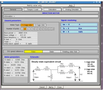
3.2.2 Modeling of Induction Motor

In this section, modeling of Induction motor element in HYPERSIM will be discussed. An induction

motor is connected at the end of series capacitor line via power transformer. Induction motor and

its power transformer being part of study area, accurate modeling of these components is required.

The general parameters of induction motor are provided in a data sheet. This datasheet

includes no-load and locked rotor test results and also specifications of the Induction Motor. From

the data, the stator resistance and inductance values and rotor resistance and inductance values are

calculated. These calculations are performed with reference to mathematical equations of no-load

(46)

Figure 3.6: Control Panel of a J-Marti Line

Calculation of Induction Motor Parameters

The constant values of induction motor are:

Applied Voltage = 6600V (line-line)

Applied Phase Voltagevph = 3810.62V (line-neutral)

(47)

No Load PF = 0.0048

Locked Rotor Current Isc = 3156A

Locked Rotor PF = 0.118

No load parametersr0 and x0 are determined using Equation 3.1 to Equation 3.6.

cosφ0= 0.048 (3.1)

φ0= 87.240 (3.2)

Im =I0sinφ0= 96.08A. (3.3)

Ic=I0cosφ0= 4.63A. (3.4)

x0 =Vph/Im = 39.65Ω (3.5)

r0=Vph/Ic= 823.004Ω (3.6)

Locked rotor parametersrl and xl are determined using Equation 3.7 to Equation 3.11:

cosφsc = 0.118 (3.7)

φsc = 83.220 (3.8)

zsc =vph/Isc = 1.207Ω (3.9)

rl=zsccosφsc = 0.142Ω (3.10)

(48)

Stator parameters rs, xs and rotor parameters rr, xr are determined by Equation 3.12 to

Equa-tion 3.14

xs =xr = 0.5xl= 0.599Ω (3.12)

xm=x0−xs= 39.051Ω (3.13)

rs=rr = (rl−rs)

xr+xm

xm

2

== 0.072Ω (3.14)

The stator and rotor resistance’s and reactances along with general parameters are

en-tered into induction motor control panel in HYPERSIM shown in Figure 3.7.

(49)

The p.u resistance and reactance values of two-winding transformer connected to the

induction motor are available in the ASPEN equivalent. These values along with primary and

sec-ondary voltages and type of transformer are entered into control panel of two-winding transformer

element in HYPERSIM. Control panel is shown in Figure 3.8.

(50)

3.2.3 Modeling of Three-Winding Transformer

In this section, another major power system element; three-winding transformer modeling in

HY-PERSIM will be discussed. These transformers are to be accurately modeled for capturing the

exact transient phenomenon. The original equipment manufacturers data for these transformers is

available in datasheets and are modeled in EMTP using ”BC-Tran block”. The data sheet contains

all the data needed for modeling the transformers except the zero-sequence test data. According to

the EMTP theory book [46], a good approximation is to take zero sequence test results as equal to

the positive sequence test results. The transformers modeled have a delta tertiary winding which

causes the excitation test to be equivalent to a short circuit test.

When all the required data entered into respective fields, EMTP generates output files.

The .pun and .out files are of interest to us. The .out file contains all the data that was entered

during the process and also the output parameters that are calculated. The .pun file contains the

calculated parameters, i.e., the resistances and the reactances of the windings. The .pun file has the

resistance R in ohms and reactance ωL in ohms. The three-winding transformer element model in

HYPERSIM accepts the winding resistance in ohms, Ω and inductance in Henry, H. The resistance

values can be obtained directly from the .pun file and the inductance of the windings is calculated

using Equation 3.15 withω being the angular frequency and f = 60Hz the system frequency.

L= X

ω (3.15)

ω= 2πf (3.16)

Figure 3.9 shows the parameters window for entering the data from the .pun file into

HYPERSIM. The data in the .pun file is in R (Ω) and X = ωL (Ω) format. The data for the

(51)

Figure 3.9: Control Panel of a Three Winding Transformer

3.2.4 Miscellaneous

All other power system components (Generators, shunt capacitor, series capacitor and MOV) in

study area are modeled using the data from the ASPEN/PSSE equivalent file. Generators are

modeled as voltage sources. The data of each component is entered into control panels of respective

power system elements in HYPERSIM. In addition to these, breaker/bus configurations at each

end of series capacitor line are also modeled in HYPERSIM.

3.2.5 Equivalent Area

Equivalent two winding transformers and equivalent π lines are connected between the boundary

buses in study area. The total number of equivalentπlines and equivalent transformers are initially

(52)

and equivalent transformers whose presence does not impact fault current value. The criteria

followed for performing sensitivity analysis is illustrated in Figure 3.10. A single line-to-ground

and three-phase-to-ground faults were applied at each terminal bus of series capacitor line. Fault

current through the line, voltages at the terminal buses of series capacitor line are captured. The

scenario is repeated by removing one equivalent line at a time and compared with values when

there is no line removed. The criteria followed for removal of an equivalent line is as follows:

1. Change in voltage is less than 1 Volt

2. Change in current is less than 10 A

3. Change in angle is less than 1 degree

This process eliminated 17 equivalent components (lines & transformers). π line and two winding

transformer elements in HYPERSIM are used to model remaining equivalentπlines and equivalent

two winding transformers using the data from ASPEN/PSSE. Because of presence of some lines &

transformer elements in HYPERSIM, four transmission lines sending and receiving end buses are

terminated on same station. To overcome this, decoupling inductor element is connected at one

end of each of these four lines. Presence of decoupling inductors made the power system unable to

produce signals at buses in the model. Different values of inductance were tried for this decoupling

inductor until signals are available at buses.

3.3 Modeling of Fault Arc

In section 3.2, modeling of power system elements in HYPERSIM was discussed. This section

discusses modeling of fault arc phenomenon in HYPERSIM. In this thesis realistic arc models

are developed and incorporated in HYPERSIM based on mathematical models developed by A.T.

(53)

start

No Outage

Apply Fault

CaptureV,I

&6 and

Remove Fault

Remove One Line

Apply Fault

CaptureV,I

&6 and

Remove Fault

Difference w.r.t No

Outage

IsV <1V,

I <5A,

6 _<₁0

Remove Line Permanently

yes

Don’t Remove Line no

Is all lines removed no

Stop yes

(54)

time varying resistor. This element is readily available in EMTP whereas in HYPERSIM, it is

required to build this time varying resistor element. To build a time varying resistor element in

HYPERSIM, User Code Model (UCM) component is used to develop this element.

UCM component is composed of a power part and a control part. The power part has

external nodes to which other power system elements are connected and control part node accepts

signals from external control blocks to perform user defined functions. A script should be developed

to build this UCM component for using it to perform user defined functions.

Fault arc phenomenon in this thesis is modeled using UCM time varying resistor and

an ideal switch. UCM time varying resistor element simulates fault arc and ideal switch is used to

simulate arc extinction and re-strike. The control node of UCM resistor element is connected to

external control blocks. These control blocks update the value of resistance in UCM time varying

resistor element for every time step.

The block diagram shown in Figure 3.11 computes primary arc resistance value. In

Figure 3.11 |i| is fault current, g is primary arc conductance and rp is primary arc resistance.

The descriptions of blocks k1 and k2 are given in Equation 3.17 and Equation 3.18 respectively.

Using the values given in Equation 3.19 and Equation 3.20, k1 and k2 are computed and used for

modeling primary arc phenomenon in HYPERSIM.

k1 1_s 1g

g

k2

|i| ₊ rp

−

(55)

k1 =

1

αVpIp

(3.17)

k2 =

Lp

αIp

(3.18)

α= 2.81×10−5, Vp= 15V /cm (3.19)

Lp = 100cm (3.20)

The block diagram shown in Figure 3.12 computes secondary arc resistance value. In

Figure 3.12 |i| is fault current,g is secondary arc conductance and rs is secondary arc resistance.

The descriptions of blocks k3 and k4 are given in Equation 3.21 and Equation 3.22 respectively.

Using the values given in Equation 3.23,k3 and k4 are computed and used for modeling secondary

arc phenomenon in HYPERSIM.

k3 1_s 1g

g

k4

|i| ₊ rp

−

Figure 3.12: Secondary Arc Block Diagram

k3=

1 75βIs

(3.21)

k4=

1

βI1.4

s

(3.22)

(56)

UCM time varying resistor element in HYPERSIM is updated with either primary arc

re-sistance value or secondary arc rere-sistance value depending on the status of series breaker. Flowchart

shown in Figure 3.13 illustrates the condition to output primary arc resistance value or secondary

arc resistance value to UCM time varying resistor element. The decision block in Figure 3.13

out-puts primary arc resistance value until the series breaker opens and outout-puts secondary arc resistance

value after series breaker opens.

rp

Is−CB−Open rs

U CM−

Resistor

yes-rs

no-rp

Figure 3.13: User Code Module Simulation Flowchart

The status (open/close) of control switch simulates arc extinction and re-strike

phe-nomenon. Flowchart shown in Figure 3.14 illustrates the condition for opening or closing of the

control switch to simulate arc extinction and arc re-strike respectively. Voltage impressed across

the arc path is compared against re-ignition voltage. When the former is less than the later, control

switch opens simulating arc extinction phenomenon and when the former is greater than the later,

control switch closes simulating arc re-strike phenomenon. When the re-ignition voltage is

perma-nently greater than recovery voltage, control switch remains open simulating permanent extinction

(57)

Varc

Varc < Vreig Vreig

Control−

Switch

yes-open

no-close

Figure 3.14: Switch Simulation Flowchart

3.4 Systematic Study Using Testview

In this section, automatic simulations of power system models using Testview software in

HY-PERSIM will be discussed. TestView is a simple powerful graphical interface designed for users

to perform automatic test sequences, automatic data analysis and graph generation [47]. It can

find automatically worst case. Testing relay for faults at different locations and different point of

incidences is a tedious process to do manually. This process can be automated in HYPERSIM

using Testview software. In Testview, scripts can be developed for applying different types of faults

at different locations and different point of incidences. Also the software outputs result in excel

format which can be used later.

Using the TestView software of HYPERSIM, a script is developed to apply faults

au-tomatically. User can define different times for switching breakers. The type of switching used is

”Uniform Type” in which user defines minimum and maximum time in seconds with reference to

t=0 of the POW for opening or closing at some random timings between specified minimum and

Test Plan for Real-Time Modeling & Simulation of Single Pole Switching Relays

ScholarWorks@UNO

ScholarWorks@UNO

Test Plan for Real-Time Modeling & Simulation of Single Pole

Test Plan for Real-Time Modeling & Simulation of Single Pole

Switching Relays

Switching Relays

Acknowledgement

Contents

List of Figures

List of Tables

Chapter 1

Introduction

1.1

Overview of Real Time Digital Simulators

1.2

A Review of Real Time Digital Simulator for Relay Testing

1.3

Overview of Single Pole Switching

1.4

A Review on Single Pole Switching Studies

1.5

Scope of Work

Chapter 2

Mathematical Formulation

2.1

Transmission Lines [1]

and past currents at both terminals. Equivalent at each terminal can therefore be

calculated in parallel.

Model for frequency dependent lines uses the same philosophy but with a more

complex equivalent.

Each half (left and right) of the line equivalents will be converted from mode to phase

form and incorporated into the corresponding substation equation to be solved with

other elements.

2.3 Substation modelling

In each substation, there are passive components interpreted as RLC elements which

can be linear or non-linear, circuit-breakers, different kinds of generation interpreted

as voltage and current sources equipped with control systems. Machines and motors

are considered as sources with control systems.

Beside control systems, other equipments are power elements working at the power

system level voltages and currents. Power elements of a substation are interconnected

together via nodes. Power elements are not simulated sequentially one by one but

rather simultaneously all together in a single equation call the

node equation

:

(9)

where

Y

is the substation admittance matrix,

V

is vector of node voltages and

I

is

vector of node currents (currents injected to nodes).

Control systems are modeled using the bloc diagram principle, either under graphic

form (Hypersim bloc diagram and Simulink bloc diagram) or coded in C/C++. Their

inputs can be node voltages and currents while their outputs can be used to control

sources and switches.

2.3.1 RLC

Hypersim, as EMTP, uses the trapezoidal integration technique, it means that

-K

M

+

YV

=

I

2.2

Mathematical Model of Three-Winding Transformers [3]

2.3

Mathematical Model of Induction Motors [4]

2.4

HYPERSIM Models for Power System Components in

Sub-station [2]

2.5

Mathematical Model of Fault Arcs [5]

Chapter 3

HYPERSIM Modeling and Relay

Design

3.1

HYPERSIM Hardware & Software Environment [6]