A High-Velocity Impact Simulation using SPH-Projection Method

A HIGH-VELOCITY IMPACT SIMULATION USING

SPH-PROJECTION METHOD

M.H. Farahani and N. Amanifard*

Department of Mechanical Engineering, Faculty of Engineering, University of Guilan P.O. Box 3756, Rasht, Iran

[email protected] - [email protected]

S.M. Hosseini

Department of Chemical and Biological Engineering, University of British Columbia Vancouver, British Columbia V6T 1Z3, Canada

[email protected]

*Corresponding Author

(Received: April 7, 2008 – Accepted in Revised Form: July 2, 2009)

Abstract In this paper, a new smoothed particle hydrodynamics (SPH) algorithm for simulation of elastic-plastic deformation of solids was proposed. The key point was that materials under high-velocity impact (HVI) behave like fluids. This led to propose a method which was similar to the so-called SPH-projection method, in which the momentum equations are solved as the governing equations. The method consisted of three steps. In the first step, a temporary velocity field was provided according to the relevant body forces. This velocity field was renewed in the second step to include the viscosity effect. Unlike the standard SPH method for elastic-plastic simulations, a Poisson equation was employed in the third step as an alternative for the equation of state in order to evaluate pressure by projecting the provisional velocity. This Poisson equation considered a trade-off between density and pressure which was utilized in the third step to impose the incompressibility effect. To illustrate the accuracy of this method a HVI problem was simulated. Results showed a good agreement with other previous works.

Keywords Smoothed Particle Hydrodynamic (SPH), High Velocity Impact (HVI), Projection Method, Meshfree Method

ﻩﺪﻴﻜﭼ

ﺍﺭﺩ ﻳ ﺭﻮﮕﻟﺍﻪﻟﺎﻘﻣﻦ ﻳ

ﺪﺟﻢﺘ ﻳﺪ ﻱ ﻫ ﺱﺎﺳﺍﺮﺑ ﻴ

ﺩﻭﺭﺪ ﻳ ﻣﺎﻨ ﻴ ﻞﺼﺘﻣ ﺕﺍﺭﺫﮏ

(SPH)

ﺍﺮﺑ ﻱ ﺒﺷ ﻴ ﺯﺎﺳ ﻪ ﻱ ﻐﺗ ﻴﻴ ﺮ

ﺎﻫﻞﮑﺷ ﻱ ﺘﺳﻻﺍ ﻴ ﮏ

-ﺘﺳﻼﭘ ﻴ ﺖﺳﺍ ﻩﺪﺷ ﻪﺋﺍﺭﺍﺕﺍﺪﻣﺎﺟ ﮏ

.

ﻠﮐ ﻪﺘﮑﻧ ﻴ ﺪ ﻱ ﺍ ﻳ ﻻﺎﺑ ﺖﻋﺮﺳﻪﺑﺮﺿ ﺭﺩ ﺩﺍﻮﻣ ﻪﮐﺖﺳﺍ ﻦ

(HVI)

ﺭﺎﺘﻓﺭ ﻱ ﺳﺪﻨﻧﺎﻣ ﻴ ﻣﻥﺎﺸﻧﺩﻮﺧﺯﺍﺕﻻﺎ ﻲ

ﺪﻨﻫﺩ

.

ﺍﻳ ﺩﻦ ﻳ ﺷﻭﺭ ﻪﺋﺍﺭﺍﻪﺑﻩﺎﮔﺪ ﻲ

ﺵﻭﺭﻪﺑﻪﮐ ﺖﺳﺍﻩﺪﺷ ﺮﺠﻨﻣ

ﻮﺼﺗ ﻳﺮ ﻱ ﻣﻞﺣ ﻢﮐﺎﺣﺕﻻﺩﺎﻌﻣﻥﺍﻮﻨﻋﻪﺑﻡﻮﺘﻨﻤﻣﺕﻻﺩﺎﻌﻣﻥﺁﺭﺩﻭﺩﺭﺍﺩﺖﻫﺎﺒﺷ ﻲ

ﺪﻧﻮﺷ

.

ﻪﺳﺯﺍﻩﺪﺷﻪﺋﺍﺭﺍﺵﻭﺭ

ﮑﺸﺗﻡﺎﮔ ﻴ ﺖﺳﺍﻩﺪﺷﻞ

.

ﻣ،ﺖﺴﺨﻧﻡﺎﮔ ﺭﺩ ﻴ

ﺘﻗﻮﻣﺖﻋﺮﺳﻥﺍﺪ ﻲ

ﻧﻪﺑﻪﺟﻮﺗﺎﺑ ﻴ

ﺎﻫﻭﺮ ﻱ ﻧﺪﺑ ﻲ ﺍﻁﻮﺑﺮﻣ ﻳ ﻣﺩﺎﺠ ﻲ ﺩﻮﺷ

.

ﺍﻳ ﻣﻦ ﻴ ﺍﻦﺘﻓﺮﮔﺮﻈﻧﺭﺩﺎﺑﻡﻭﺩﻡﺎﮔﺭﺩﺖﻋﺮﺳﻥﺍﺪ ﺪﺠﺗﺖﺟﺰﻟﺮﺛ

ﻳ ﻣﺪ ﻲ ﺩﻮﺷ

.

ﺩﺭﺍﺪﻧﺎﺘﺳﺍﺵﻭﺭﻑﻼﺧﺮﺑ

SPH

ﺍﺮﺑ ﻱ

ﺒﺷ ﻴ ﺯﺎﺳﻪ ﻱ ﺎﻫ ﻱ ﺘﺳﻻﺍ ﻴ ﮏ

-ﺘﺳﻼﭘ ﻴ ﺯﺍ،ﮏ ﻳ ﺎﺟﻥﺍﻮﻨﻋﻪﺑﻡﻮﺳﻡﺎﮔﺭﺩﻥﻮﺳﺍﻮﭘﻪﻟﺩﺎﻌﻣﮏ ﻳ

ﺰﮕ ﻳﻨ ﻲ ﺍﺮﺑ ﻱ ﺖﻟﺎﺣﻪﻟﺩﺎﻌﻣ

ﺍﺮﺑ ﻱ ﻮﺼﺗﺎﺑ،ﺭﺎﺸﻓﻪﺒﺳﺎﺤﻣ ﻳ

ﺘﻗﻮﻣﺖﻋﺮﺳﻥﺩﺮﮐﺮ ﻲ

ﻣﻩﺩﺎﻔﺘﺳﺍ، ﻲ

ﺩﻮﺷ

.

ﺍﻳ ﺍﻪﻧﺯﺍﻮﻣﻥﻮﺳﺍﻮﭘﻪﻟﺩﺎﻌﻣﻦ ﻱ

ﺑﺍﺭ ﻴ ﻟﺎﮕﭼﻦ ﻲ

ﺭﺎﺸﻓﻭ ﺍ ﻳ ﻣﺩﺎﺠ ﻲ ﺍﺮﺑﻡﻮﺳﻡﺎﮔﺭﺩﻥﺁﺯﺍﻪﮐﺪﻨﮐ ﻱ

ﺬﭘﺎﻧﻢﮐﺍﺮﺗﻞﻤﻋ ﻳﺮ

ﻱ ﻣﻩﺩﺎﻔﺘﺳﺍ ﻲ ﺩﻮﺷ

.

ﺍﺮﺑ ﻱ ﺘﺳﺭﺩﻥﺩﺍﺩﻥﺎﺸﻧ ﻲ

ﺍﻳ ﺵﻭﺭﻦ ﻳ ﻪﻠﺌﺴﻣﮏ

HVI

ﺒﺷ ﻴ ﺯﺎﺳﻪ ﻱ ﺖﺳﺍﻩﺪﺷ

.

ﺎﺘﻧ ﻳ ﺑﻮﺧﻖﻓﺍﻮﺗﺞ ﻲ

ﺎﻫﺭﺎﮐﺎﺑﺍﺭ ﻱ ﻣﻥﺎﺸﻧﻪﺘﺷﺬﮔ ﻲ

ﺪﻫﺩ

.

1. INTRODUCTION

Lagrangian Finite Element (LFE) method and Eulerian approach have been the most dominant methods for solving problems which have dealt with the simulation of solid deformation since the 1980s. Both methods were used in a wide range of

generally limited to problems where the amounts of deformation are small, because they suffer from mesh distortion problem which is created as a result of grid entanglement. Although Eulerian method, in which the grid remains fixed in space, is free from the mesh distortion problem, but it needs to use sophisticated techniques to track the material interface which produces a complex challenge. Thus, developing efficient methods which are able to avoid these deficiencies have been at the center of attention. On the one hand, this has led to a group of combined Eulerian and Lagrangian methods such as Arbitrary Lagrangian Eulerian (ALE) approach, and, on the other hand, has developed a new class of methods which are called meshless or particle methods. Smoothed Particle Hydrodynamics (SPH) is one of these meshless methods and first adapted to model the dynamic response of solids in 1991 by Libersky, et al [1]. Basically, SPH is a grid-free computational technique for equations of fluid dynamics in Lagrangian framework which initially was proposed by Lucy [2] and separately by Gingold, et al [3] in 1977. Although the basic application of this method was first in astrophysics, nowadays this method is used in variety of applications including incompressible fluid flow, multiphase flow, heat and mass transfer, elasticity and fracture, etc. A very good review of this method and its application is presented by Monaghan [4]. In spite of rather extraordinary results, first applications of SPH were somehow crude, since there were some instabilities and deficiencies in the obtained results [5]. Problems such as tensile instability, zero energy mode and boundary condition treatment were of these problems for which remedies have been proposed [6-15]. Progressive improvements of this method have led it into a wide range of applications which introduces SPH as a versatile computational method. This mainly comes from its simplicity and the ability to extend it to new complex physics [16].

In the field of impact engineering, distinctive futures are demonstrated in association with SPH. Surface tracking is treated according to the Lagrangian nature, while the inherent mesh-free character makes it suitable for simulations including large strain. In this way, SPH is used widely in HVI and penetration simulations [17]. A constitutive model as well as a proper equation of state (usually

Mie-Gruneisen equation of state) is utilized in SPH for such simulations. Meanwhile, artificial viscosity is usually used to control both the numerical instability and shock wave capturing [17].

2. GOVERNING EQUATIONS

The governing equations for an elastic body are as follow:

j x

ij 1 i g Dt

i Du

∂ σ ∂ ρ +

= (1)

i x

i u Dt

D

∂ ∂ ρ − = ρ

(2)

Where t is the time and ρ is the density. Superscripts i and j (and k) are free indices. Moreover, _ui_{, x}j_{, and g}i _{are velocity vector,} position vector, and body force per unit mass, respectively and _σij _{is the stress tensor which can} be written as:

ij S ij P

ij_{=− δ +}

σ (3)

Where _Sij _{is the deviatoric stress tensor. By} assuming linear elastic theory and considering Hooke’s law, the deviatoric stress can be presented as follows [13]:

kj S ik jk ik S ij ij 3 1 ij 2 t d

ij S

d _{⎟+ ω +ω}

⎠ ⎞ ⎜

⎝

⎛_{ε − δ ε} μ

= & & (4)

Where μ is the shear modulus. The strain rate tensor_ε&ij_{, and rotation tensor ω}ij _{are defined as} follow:

⎟ ⎟ ⎠ ⎞ ⎜

⎜ ⎝ ⎛

∂ ∂ + ∂ ∂ = ε

i x

j u j x

i u 2 1 ij

& (5)

⎟ ⎟ ⎠ ⎞ ⎜

⎜ ⎝ ⎛

∂ ∂ − ∂ ∂ = ω

i x

j u j x

i u 2 1

ij ₍₆₎

Combining the Equations 1 and 3 yields:

j x

P 1 j x

ij S 1 i g Dt

i Du

∂ ∂ ρ − ∂ ∂ ρ +

= (7)

To model the plastic behavior of materials an additional yield criterion and a flow rule is required. The yield criterion determines the stress

state when the plastic flow occurs (yielding), while the flow rule specifies the increment of the plastic strain once the material has yielded. With most materials, there is a gradual transition from elastic to plastic behavior; therefore, defining the point at which plastic deformation begins is also difficult during experiments. For the present work, the von Mises yield criterion has been employed. For two dimensions, the criterion is defined as [25]:

2 0 Y 3 2 2 xy S 2 2 y S 2 x

S + + ≤ (8)

Where Y₀ is the yield stress. For the sake of simplicity, and in order to permit a comparison with the simulations performed by others [17,25], an elastic-perfectly plastic flow rule has been selected. Thus, if inequality (8) is not satisfied, then material undergoes the plastic flow, and therefore, each stress component should be rescaled to lie on the yield surface. According to the literature [25] the radial return method is used. Based on this method, each stress component is radially rescaled to lie on the yield surface by being multiplied by the rescaling factor as follows:

2 xy S 2 2 y S 2 x S

0 Y 3 2

+ +

(9)

3. METHODOLOGY

3.1. Basic Concepts

SPH is a mesh-free method based on the interpolation theory in which matter is divided into a set of interpolation points, so-called particles. These particles carry the material properties such as density, velocity, pressure, stress and etc. Integral interpolation among these particles using a kernel function approximates the field variables.

Supposing A as a field variable of the spatial coordinates, the exact integral representation of A is as follows:

( )

( ) (

δr r

)

dr Ω

r A r

A =

∫

′ − ′ ′ (10)

the computational domain. This can be represented by integral interpolation of quantity A as:

( )

( ) (

Wr r,h

)

dr

Ω

r A r

A = ∫ ′ − ′ ′ (11)

Where the angle bracket 〈 〉 denotes kernel approximation, h is the smoothing length proper to kernel function and W represents the effective width of the kernel. The kernel has the following properties [4]:

(

)

(

) (

)

⎪ ⎩ ⎪ ⎨ ⎧ ′ − = ′ − → ∫ − ′ ′= r r δ h , r r W 0 hlim V 1 r d h , r r W (12)

Several kernel functions have been proposed for the SPH method. The most frequently used kernel is the cubic spline kernel, which is written as follows [4]: ⎪ ⎪ ⎪ ⎩ ⎪⎪ ⎪ ⎨ ⎧ ≥ < ≤ − < ≤ + − × ν κ = 2 s 0 2 s 1 3 ) s 2 ( 4 1 1 s 0 3 s 4 3 2 s 2 3 1 h ) h ,r (

W (13)

Where

h r

s= , ν is number of dimensions and κ is normalization constant with the values:

π π 1 , 7 10 , 3 2

for one, two and three dimensions,

respectively. This kernel has compact support which is equal to2h; it means that interactions vanish forr>2h. The dominant error term in the integral interpolant is O(h2) _[16].

If A(r′) is known only at a discrete set of N points r₁,r₂,...,r_N then the interpolation of quantity A can be approximated by a summation interpolant as follows [4]:

( )

N_{b 1} A_bW

(

r r,h

)

b ρ b m r h

A =_{∑ =} − ′ (14)

Where the summation index b denotes a particle label and particle b carries a mass m_b at position

b

r , a density ρ_b and a velocity v_b. The value of A at b−th particle is shown by A_b. For the cubic spline kernel, the summation is over the particles that lie within a circle of radius 2h centered at r. Derivative of A with respect to x is given by the following equation [16]:

(

)

∑ ∂ ∂ − ρ Φ Φ = ⎟ ⎠ ⎞ ⎜ ⎝ ⎛ ∂ ∂ b x ab W a A b A b b b m a 1 a x

A ₍₁₅₎

Where Φ is any differentiable function and

(

,h

)

W

W_ab = ra−rb′ .

3.2. Gradient and Divergence

The gradient and divergence operators need to be formulated in this SPH algorithm. In the current work, the following commonly used forms are employed for gradient of a scalar A and divergence of a vector u

[19,26]:

ab W a

b _b2

b A 2 a a A b m A a a 1 _∇ ∑ ⎟⎟ ⎟ ⎠ ⎞ ⎜⎜ ⎜ ⎝ ⎛ ρ + ρ = ∇ ρ (16) ab W a

b _b2

i a u 2 a i a u b m i a u . a a

1 _⋅∇

∑ ⎟ ⎟ ⎟ ⎠ ⎞ ⎜ ⎜ ⎜ ⎝ ⎛ ρ + ρ = ∇

ρ (17)

Where ∇_a represents the gradient with respect to coordinates of particle a.

3.3. Laplacian Formulation A simple way to

formulate the Laplacian operator is to envisage it as dot product of the divergence and gradient operators. This approach proved to be problematic as the resulting second derivative of the kernel is very sensitive to particle disorder and can easily lead to pressure instability and decoupling in the computation due to the co-location of the velocity and pressure. In this paper, the following alternative approach is adopted [19,20]:

∑ + ∇ ⎟ ⎠ ⎞ ⎜ ⎝ ⎛ ₊ = ⎟⎟ ⎠ ⎞ ⎜⎜ ⎝ ⎛ _∇ ∇

b 2 _η2

ab r ab W a . ab r ab A 2 b ρ a ρ 8 b m a A ρ 1

. (18)

3.4. Variable Smoothing Length Using a

variable smoothing length is essential for problems that material undergoes an expansion or compression. In HVI problems, local compression in impact zone and expansions such as debris cloud, make the application of variable smoothing length inescapable. If such problems are treated with a constant smoothing length approach, as an example for an expansion condition, after certain analysis time, very few neighbor particles will be found for a particle that at the beginning of the analysis was well covered and vice versa [27]. Various methods have been proposed to adjust the smoothing length in order to enhance the accuracy and flexibility of the SPH method. These methods are usually based on the variation of density. In this work, the method suggested by Monaghan [16] is employed. In this way variable smoothing length is satisfied according to the following equation:

dt ln d 1 dt

h ln

d ρ

ν −

= (19)

Where ν is the number of dimensions.

4. SOLUTION ALGORITHM

Projection methods are fractional step methods in which incompressibility is satisfied considering the prediction-correction steps [28]. In this paper the authors follow an explicit algorithm which is combined of three steps [19]. The first two steps play the role of prediction part of the pressure projection method and the third one is a correction. These three steps are according to the three parts in the right hand side of the momentum Equation 7 and combination of third part with continuity Equation 2.

4.1. First Step In the first step of this algorithm,

the momentum equation is solved in the presence of the body forces neglecting all other forces. The computed intermediate velocity is used in the second step to calculate the divergence of the deviatoric stress tensor as:

t i g i

t t u i

u~ = _−Δ + Δ (20)

4.2. Second Step In this step, the divergence of

the deviatoric stress tensor is calculated (instead of the calculation of divergence of shear stress tensor in a fluid dynamic algorithm) based on the intermediate velocity field computed in the first step. In this way, the deviatoric stress tensor is calculated according to the constitutive Equation 4. The divergence of the deviatoric stress tensor is a vector _Ti _{which is given by the following} equation:

ab W a 2 b

ρ

ij b S 2 a

ρ

ij a S

b b

m i T a j x

ij S

ρ

1 _⋅∇

⎟ ⎟ ⎟ ⎠ ⎞ ⎜

⎜ ⎜ ⎝ ⎛

+ ∑

= = ⎟ ⎟ ⎠ ⎞ ⎜ ⎜ ⎝ ⎛

∂

∂ ₍₂₁₎

Where

⎟ ⎠ ⎞ ⎜

⎝ ⎛ ₋ =

∇ xi_a x_bj ab

r 1 ab dr

dW ab W

a (22)

The vector _Ti _{is used to update the temporary} velocity filed as follows:

t i T t i g i

t t u t i T i u~ i u

~~ _{+ Δ + Δ}

Δ − = Δ +

= (23)

This temporary velocity field is employed to move particle into a new temporary position as the following equation:

t i u ~~ i

t t x i

x~ = _−Δ + Δ (24)

4.3. Third Step There was no constraint to

impose the incompressibility effect in both previous steps, thus particle movement changed the density of the particles. These density variations can be calculated with the help of the continuity equation. Monaghan [16] discussed different kinds of continuity equations in SPH framework. Using Equation 15, two useful forms of continuity equations are defined. Choosing

1 =

Φ gives:

ab W a i b u i a u b

b m a a dt

d _{∑ ⎟⋅∇}

⎠ ⎞ ⎜

⎝

⎛ ₋

ρ ρ = ⎟ ⎠ ⎞ ⎜ ⎝

⎛ ρ ₍₂₅₎

while choosing Φ=ρ yields:

ab W a b

i b u i a u b m a dt

d _∇

∑ ⎟⋅

⎠ ⎞ ⎜

⎝ ⎛ ₋ =

⎟ ⎠ ⎞ ⎜ ⎝

It is demonstrated that when the system involves two or more materials with the density ratio ≥ 2 in contact, Equation 25 is more accurate in comparison with Equation 26 [16]. This is a common condition in HVI problems; thus, in our simulations Equation 25 is the base of density computations.

Considering the continuity Equation 25, a temporary density is achieved. When two particles approach each other, their relative velocity and the gradient of kernel function have same signs, therefore

(

dρ~ Dt

)

_a will be positive and ~ρ_a will increase. Consequently, this will produce a repulsive force between the approaching particles, and vice versa. This interaction based on the relative velocity of the particles and the resulting coupling between the pressure and density will enforce incompressibility in the solution procedure.

The velocity field _uˆi _{which is needed to restore} the density of particles to their original value is calculated. To do this, in the third step of the algorithm, the momentum equation with the pressure gradient term as a source term is combined with the continuity Equation 2 as follows:

0 j x j uˆ t ~ 0 0 1 ₌ ∂ ∂ + Δ ρ − ρ

ρ (27)

t P ~ 1 i

uˆ _⎟⎟Δ

⎠ ⎞ ⎜⎜ ⎝ ⎛ ∇ ρ −

= (28)

To obtain the following Poisson equation for pressure Equation 29 is developed as follows:

2 t 0 ~ 0 P ~1 . Δ ρ ρ − ρ = ⎟⎟ ⎠ ⎞ ⎜⎜ ⎝ ⎛ _∇ ρ

∇ (29)

Equation 29 can be discretized according to Equation 18 to obtain the pressure of each particle as the following equation:

⎟⎟ ⎟ ⎟ ⎠ ⎞ ⎜⎜ ⎜ ⎜ ⎝ ⎛ + ∇ ∑ + ⎟⎟ ⎟ ⎟ ⎠ ⎞ ⎜⎜ ⎜ ⎜ ⎝ ⎛ + ∇ ∑ + + − = 2 η 2 ab r ab W a . i ab x

b(ρ_a ρ_b)2

b m 8 2 η 2 ab r ab W a . i ab x b P

b(ρ_a ρ_b)2

b m 8 2 Δt 0 ρ a ρ ~ 0 ρ a P (30)

using this value for the pressure of each particle

one can calculate _uˆi _{according to Equation 28 and} 16 as follows:

ab W a ) 2 b b P 2 a ~a P ( b b m t i a uˆ ∇ ρ + ρ ∑ Δ −

= (31)

Finally, overall velocity of each particle at the end of time step will be obtained as:

i uˆ i u ~~ i t t

u _+Δ = + , (32)

and the final positions of particles are calculated using a central difference scheme in time based on the following equation:

) i t t u i t u ( 2 t i t t x i t

x = _−Δ +Δ + _−Δ (33)

5. TEST CASE

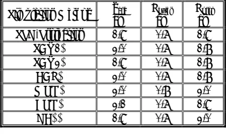
The impact problem studied byHowell, et al [25] using a Lagrangian finite-volume Godunov scheme is considered as a benchmark. This problem was also studied by Mehra, et al [17] with different artificial viscosities defined for SPH simulations as well as a contact SPH method. The problem involves a 2D HVI of a cylindrical projectile with a plate. The projectile is made of aluminum (Al) or steel with a 10 mm diameter which moves with an initial speed of 3.1 km/s toward target, while the target is made of Al with 2 mm thickness. Material properties are tabulated in Table 1. In our simulations we assumed there are no external body forces. Inter-particle distance (Δx) is set to be 0.1 mm and simulations are started with 1.5

x

h ₌

Δ , and

Δt = 0.1 × 10-9_{s. The projectile includes 8012} particles while 10000 particles are within the target. A schematic view of the initial location of the particles is shown in Figure 1a.

6. RESULTS AND DISCUSSIONS

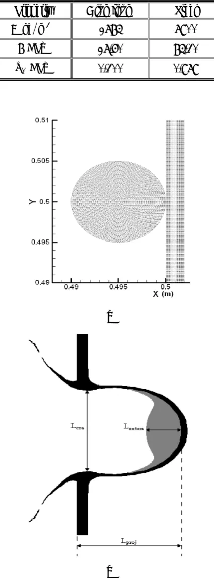
Also, the obtained results are tabulated in Tables 2 and 3 and compared with the results which were reported by Howell and Ball based on Lagrangian finite-volume Godunov scheme [25], as well as different SPH schemes [17] where dcra is the crater diameter, Lexten is the longitudinal extension of the projectile, and Lproj is the longitudinal progress of the projectile through the target (Figure 1b). All the above values are reported in 8 μs after impact. CON is based on the Riemann approach which is exempt of artificial viscosity [29,30]. SAV1 and SAV2 are purely based on the standard SPH method, but differ in constant values of artificial viscosity. BAL and MON are also based on the standard SPH but their artificial viscosity is modified by Balsara [31], and Morris, et al [32], respectively. Lengths are resolved in SPH ≥ 2h, and are quoted here to 0.1 cm. Mehra, et al [17] reported a tendency to form clamp for all standard SPH simulations of similar HVI problems (AL-AL and steel-AL) as a result of tensile instability, while such phenomenon was not reported for CON. Thus, they concluded that CON is the best SPH method in their HVI simulations which had shown the closest agreement with the results of HB. It is clear from Figures 2 and 3 that the pressure-projection method shows no tendency to clamp formation. This confirms the SPH-projection method by simulating the impact of an elastic ring with a rigid wall. It will be more interesting if we notice that unlike the standard SPH method, no remedy is introduced to eliminate the tensile instability. Furthermore, comparing the geometrical results of SPH-projection and CON, closest agreement is provided by SPH-projection method with the results reported by HB (the main reference). These superb results are obtained according to the pressure that is computed using the pressure Poisson Equation 30, however, the generated pressure at the center of the projectile, 1

μs after impact (also reported in [17]) was almost half of the pressure reported by Howell, et al [25] (18.6 GPa for Al-Al and 27.9 GPa for steel-Al). This reality comes from the fact that the proposed algorithm is slightly dissipative. Therefore, it seems necessary to make a compromise between the dissipation terms and evaluation of the pressure to achieve a higher accuracy. One of the best choices is to extend a more accurate projection method into SPH framework. It is important to consider some other main differences between the proposed

SPH-TABLE 1. Properties of Al and steel used for HVI simulations.

Property Aluminum Steel )

m kg

( 3

ρ 2785 7900

) Pa G (

μ _{27.60 85.30}

) Pa G (

Y₀ 0.300 0.979

(a)

(b)

projection algorithm and the standard SPH algorithms with concentrating on not using the artificial viscosity. As the first difference, energy equation is simply neglected in our simulations. It is noticeable that the other SPH methods often use common equations of state such as Mie-Gruneisen equation of state, which highly depends on the energy equation. Moreover, equations of state are based on statistical mechanics and are only valid over a limited range of its material

dependent parameters. Therefore, several equations of state need to be available to) use in any numerical algorithm. Consequently, the pressure Poisson equation is employed instead of any equations of state in the present proposed algorithm so that the computed pressure values are completely sensitive to any density variations.

The results provided in this section are not just a comparison between different numerical methods and schemes, but also include the experimental

(a) (b) (c) (d)

Figure 2. Impact of an Al projectile with an Al target at 3.1 km/s. (upper half: SPH-projection, lower half: lagrangian finite-volume Godunov scheme [25]), (a) 2μs,(b) 4μs, (c) 6μs and (d) 8μs.

(a) (b) (c) (d)

results. Firstly, close agreement of the obtained results with published simulation results gives a sense of confidence in our results. Besides, the comparisons bear interesting information regarding the proposed algorithm and the previously proposed methods.

7. CONCLUSION

This paper proposes an alternative SPH algorithm for simulating HVI problems. The algorithm is composed of three steps which plays the role of a pressure-correction method. In the first two steps, a provisional velocity is provided which is projected in the third step to impose the compressibility

constraint. In this way, the artificial viscosity is neglected and the Poisson equation is employed without any usage of equations of state. Tensile instability is treated naturally while dissipation terms decrease the evaluated pressure. Comparing the computed geometrical results of the presented method with other SPH methods shows adequate agreements [17,25].

8. NOMENCLATURE

A A Typical Field Variable g Gravity Force Per Unit Mass

h Smoothing Length

m Mass P Pressure

r Position Tensor

S Deviatoric Stress Tensor s Normalized Position Variable

T Divergence of Deviatoric Stress Tensor t Time

u Velocity Vector

W Kernel Function

Y0 Yield Stress

σ Stress Tensor

ρ Density

δ Dirac Delta Function

μ Shear Modulus

ε Strain Rate Tensor

ω Rotation Tensor

Ω Computational Domain

ν Number of Dimensions

κ Normalization Constant

Φ A Differentiable Function

η A Small Number to Avoid Singularity

Subscripts

a Target Particle Index

b Neighborhood Particle Index

t Time Index

Δt Time Step

Superscripts

i Normal in x-Direction j Normal in y-Direction ~,≈ Temporal Variables

^ Field Variables

TABLE 2. Comparison of the geometrical results of the impact of an Al projectile with an Al target at 3.1 km/s.

Simulation Method dcra (cm)

Lexten (cm)

Lproj (cm)

SPH-Projection 1.9 0.7 1.9

SAV1* 2.0 0.7 1.8

SAV2* 1.9 0.7 1.8

BAL* 2.0 0.7 1.8

MON* 2.0 0.8 2.0

CON* 2.1 0.7 1.9

HB** 1.9 0.7 2.0

* Results are quoted from [17] ** Results are quoted from [25]

TABLE 3. Comparison of the geometrical results of the impact of a steel projectile with an Al target at 3.1 km/s.

Simulation method dcra (cm) Lproj (cm) SPH-Projection 1.5 2.2

SAV1* 1.9 2.1

SAV2* 1.9 2.1

BAL* 1.8 2.2

MON* 1.8 2.2

CON* 1.7 2.2

HB** 1.6 2.3

9. REFERENCES

1. Libersky, L.D. and Petschek, A.G., “Smoothed Particle Hydrodynamics with Strength of Materials”, Proceedings of the Next Free Lagrange Conference, In Trease, H.,

Fritts, J. and Crowley, W., (Eds), Springer: New York, U.S.A., Vol. 395, (1991), 248-257.

2. Lucy, L.B., “A Numerical Approach to the Testing of the Fission Hypothesis”, Astron. J., Vol. 82, (1977),

1013-1024.

3. Gingold, R.A. and Monaghan, J.J., “Smoothed Particle Hydrodynamics: Theory and Application to Non-Spherical Stars”, Mon. Not. R. Astron. Soc., Vol.181,

(1977), 375-89.

4. Monaghan J.J., “Smoothed Particle Hydrodynamics”,

Ann. Rev. Astron. Astrophys., Vol. 30, (1992), 543-574. 5 Randles, P.W. and Libersky, L., “Smoothed Particle

Hydrodynamics Some Recent Improvements and Applications”, Comput. Methods Appl. Mech. Eng.,

Vol. 139, (1996), 375-408.

6. Swegle, J., Hicks, J. and Attaway, S., “Smoothed Particle Hydrodynamics Stability Analysis”, J. Comput. Phys.,

Vol. 116, (1995), 123-34.

7. Dyka, C.T. and Ingel, R.P., “An Approach for Tension Instability in Smoothed Particle Hydrodynamics (SPH),

Computers and Structures, Vol. 57, (1995), 573-580.

8. Johnson, G.R., Stryk, R.A. and Beissel, S.R., “SPH for High Velocity Impact Computations”, Comput. Methods. Appl. Mech. Eng., Vol. 139, (1996), 347-73.

9. Dyka, C.T., Randies, P.W. and Ingel, R.P., “Stress Points for Tension Instability in Smoothed Particle Hydrodynamics”, International Journal for Numerical Methods in Engineering, Vol. 40, (1997), 2325-2341. 10. Chen, J.K., Beraun, J.E. and Jih, C.J., “An improvement

for Tensile Instability in Smoothed Particle Hydrodynamics”, Computational Mechanics, Vol. 23,

(1999), 279-287.

11. Randles, P.W. and Libersky, L.D., “Normalized SPH with Stress Points”, Int. J. Numer. Meth. Engng., Vol. 48, (2000), 1445-1462.

12. Monaghan, J.J., “SPH Without a Iensile Instability”, J. Comput. Phys.,Vol. 159, (2000),290-311.

13. Gray, J., Monaghan, J.J. and Swift, R.P., “SPH Elastic Dynamics”, Comput. Methods Appl. Mech. Eng., Vol.

190, (2001),6641-6662.

14. Bonet, J. and Kulasegaram, S., “Remarks on Tension Instability of Eulerian and Lagrangian Corrected Smooth Particle Hydrodynamics (CSPH) Methods”, Int. J. Numer. Meth. Engng., Vol. 52, (2001), 1203-1220.

15. Vidal, Y., Bonet, J. and Huerta, A., “Stabilized Updated Lagrangian Corrected SPH for Explicit Dynamic Problems”, Int. J. Numer. Meth. Engng., Vol. 69,

(2007), 2687-2710.

16. Monaghan, J.J., “Smoothed Particle Hydrodynamics”,

Rep. Prog. Phys., Vol. 68, (2005), 1703-1759.

17. Mehra, V. and Chaturvedi, S., “High Velocity Impact of Metal Sphere on thin Metallic Plates: A Comparative

Smooth Particle Hydrodynamics Study”, J. Comput. Phys., Vol. 212, (2006), 318-337.

18. Liu, G.R. and Liu, M.B., “Smooth Particle Hydrodynamics, A Meshfree Particle Method”, 1nd _{ed. World Scientific,} (2003), 309-340.

19. Hosseini, S.M., Manzari, M.T. and Hannani, S.K., “A Fully Explicit Three Step SPH Algorithm for Simulation of Non-Newtonian Fluid Flow”, Int. J. of Numerical Methods for Heat and Fluid Flow, Vol. 17,

(2007), 715-735.

20. Cummins, S.J. and Rudman, M., “An SPH Projection Method”, J. Comp. Physics, Vol. 152, (1999), 584-607. 21. Lo, E.Y.M. and Shao, S., “Simulation of Near-Shore

Solitary wave Mechanics by an Incompressible SPH Method”, Applied Ocean Research, Vol. 24, (2002),

275-286.

22. Shao, S. and Lo, E.Y.M., “Incompressible SPH Method for Simulating Newtonian and non-Newtonian flows with a Free Surface”, Advances in Water Resources,

Vol. 26, (2003), 787-800.

23. Hosseini, S.M. and Amanifard, N., “Presenting a Modified SPH Algorithm for Numerical Studies of Fluid-Structure Interaction Problems”, International

Journal of Engineering, Trans B: Applications, Vol.

20, (2007), 167-178.

24. Antoci, C., Gallati, M. and Sibilla, S., “Numerical Simulation of Fluid-Structure Interaction by SPH”,

Computers and Structures, Vol. 85, (2007), 879-890.

25. Howell, B.P. and Ball, G.J., “A Free-Lagrange Augmented Godunov Method for the Simulation of Elastic-Plastic Solids”, J. Comput. Phys., Vol. 175,

(2002),128-167.

26. Colagrossi, A. and Landrini M., “Numerical Simulation of Interfacial flows by Smoothed Particle Hydrodynamics”,

J. Comput. Phys., Vol. 191, (2003), 448-475.

27. Bonet, J. and Rodriguez-Paz, M.X., “Hamiltonian Formulation of the Variable-h SPH Equations”, J. Comput. Phys., Vol. 209, (2005), 541-558

28. Guermond, J.L., Minev, P. and Shen, J., “An Overview of Projection Methods for Incompressible Flows”,

Comput. Methods Appl. Mech. Engrg., Vol. 195,

(2006), 6011-6045.

29. Parshikov, A., Medin, S.A., Loukashenko, I. and Milekhin, V., “Improvements in SPH Method by Means of Inter-Particle Contact Algorithm and Analysis of Perforation Tests at Moderate Projectile Velocities”,

Int. J. Impact Eng., Vol. 24, (2000), 779-796.

30. Parshikov, A. and Medin, S.A., “Smoothed Particle Hydrodynamics using Interparticle Contact Algorithms”,

J. Comput. Phys., Vol. 180, (2002) 358-382.

31. Balsara D.S., “Von Neumann Stability Analysis of Smoothed Particle Hydrodynamics-Suggestions for Optimal Algorithms”, J. Comput. Phys., Vol. 121,

(1995), 357-372.