A Boundary Elements and Particular Integrals Implementation for Thermoelastic Stress Analysis

A BOUNDARY ELEMENTS AND PARTICULAR

INTEGRALS IMPLEMENTATION FOR

THERMOELASTIC STRESS ANALYSIS

M. Hemayati

Surface Effect Research Institute, Shahid Charmin Boulevard Shiraz, Iran

G. Karami

Department of Mechanical Engineering, School of Engineering, Shiraz University Shiraz, Iran, [email protected]

(Received: October 2, 2000 - Accepted in Revised Form: August 20, 2001)

Abstract A formulation and an implementation of two-dimensional Boundary Element Method (BEM) analysis for steady state, uncoupled thermoelastic problems is presented. This approach differs from other treatments of thermal loads in BEM analysis in which the domain integrals due to the thermal gradients are to be incorporated in the analysis via particular-integrals. Thus unlike Finite Elements or Field Boundary Elements algorithms the domain discretization becomes unnecessary. The algorithm and the formulation are implemented in a general purpose, multi-region two-dimensional analysis. Isoparametric quadratic elements are employed to represent the geometry and the field variables. Examples are presented to demonstrate the accuracy and versatility of the method.

Key Words Thermoelasticity, Boundary-Element-Method, Particular Integrals

ﻩﺪﻴﻜﭼ

ﺖﺳﺍﻩﺪﻳﺩﺮﮔﻪﺋﺍﺭﺍﻪﻟﺎﻘﻣﻦﻳﺍﺭﺩﻪﺘﻴﺴﻴﺘﺳﻻﺍﻮﻣﺮﺗﻱﺪﻌﺑﻭﺩﻞﺋﺎﺴﻣﻱﺍﺮﺑﻱﺯﺮﻣﺮﺻﺎﻨﻋﺪﻳﺪﺟﺵﻭﺭﻚﻳ

.

ﺎﺑ ﻥﺁ ﺕﻭﺎﻔﺗ ﻭ ﻪﺘﺷﺍﺩ ﺩﺮﺑﺭﺎﻛ ﻪﻨﻣﺍﺩ ﺭﺩ ﺍﺭﺬﮔ ﻭ ﺖﺧﺍﻮﻨﻜﻳ ﻱﺎﻣﺩ ﻊﻳﺯﻮﺗ ﺎﺑ ﻞﺋﺎﺴﻣ ﻞﺣ ﻱﺍﺮﺑ ﻩﺪﺷ ﻪﺋﺍﺭﺍ ﺵﻭﺭ

ﻲﺗﺭﺍﺮﺣﻱﺎﻫﻭﺮﻴﻧ ﺯﺍﻲﺷﺎﻧ،ﻪﻨﻣﺍﺩﻱﻭﺭ ﻱﺎﻬﻟﺍﺮﮕﺘﻧﺍ ﻪﻜﺘﺴﻧﺁﺭﺩ ﻲﻠﺒﻗﻱﺎﻬﺷﻭﺭ

ﺭﺩﺹﻮﺼﺨﻣ ﻱﺎﻬﻟﺍﺮﮕﺘﻧﺍﻚﻤﻛ ﻪﺑ

ﻲﻣﻪﺘﻓﺮﮔﺮﻈﻧﺭﺩﻱﺯﺮﻣﺮﺻﺎﻨﻋﻢﺘﺴﻴﺳ ﺪﻧﻮﺷ

. ﻑﺭﺎﻌﺘﻣﻱﺎﻬﺷﻭﺭﺎﻳﻭﺩﻭﺪﺤﻣﺮﺻﺎﻨﻋﺵﻭﺭﻑﻼﺧﺮﺑﺐﻴﺗﺮﺗﻦﻳﺪﺑ

ﻥﺎﻤﻟﺍ ﻪﺑ ﻱﺯﺎﻴﻧ ،ﻱﺯﺮﻣ ﺮﺻﺎﻨﻋ

ﺩﻮﺑ ﺪﻫﺍﻮﺨﻧ ﻪﻨﻣﺍﺩ ﻱﺪﻨﺑ

.

ﺭﺎﻜﺑ ﺰﻴﻧ ﻪﻴﺣﺎﻧ ﺪﻨﭼﻞﻣﺎﺷ ﻱﺎﻬﻤﺘﺴﻴﺳﻱﺍﺮﺑ ﺵﻭﺭ ﻦﻳﺍ

ﻲﻣ

ﻳﺁ ﻭﻡﻭﺩﻪﺟﺭﺩ ﻱﺎﻬﻧﺎﻤﻟﺍﺯﺍ ﻥﺁ ﺭﺩ ﻭﺩﻭﺭ

ﻩﺪﺷﻩﺩﺎﻔﺘﺳﺍ ﻢﺴﺟ ﻪﺳﺪﻨﻫ ﻭﻊﺑﺍﻮﺗ ﻥﺩﺍﺩ ﻥﺎﺸﻧﻱﺍﺮﺑ ﻚﻳﺮﺘﻣﺍﺭﺎﭘﻭﺰ

ﺖﺳﺍ

.

ﺖﺳﺍﻩﺪﺷﻪﺋﺍﺭﺍﻲﻳﺎﻬﻟﺎﺜﻣ،ﺵﻭﺭﺖﻗﺩﻭﻲﻳﺎﻧﺍﻮﺗﻥﺩﺍﺩﻥﺎﺸﻧﺭﻮﻈﻨﻤﺑ

.

1. INTRODUCTION

Usually the thermoelastic problems may be solved using small modifications to the pure elastic formulations by treatment of the temperature gradients as a kind of body forces. In BEM analysis this will include an extra domain integral to the resulted boundary-only integrals of elastic formulation. Hence the domain of the problem should be discretized for the sole implementation of thermal forces. This obviously would loose the benefits of boundary-only BEM analysis. To avoid the domain discretization several transforming schemes are proposed and implemented. Other methods would include

Brebbia [9] and Neves and Brebbia [10] have used Dual Reciprocity and Multiple Reciprocity Methods (DRM, and MRM). Other solutions include the use of Papkovich and Neuber stress functions (see for example Kuhn [11]). Also, Sharp and Crouch [12] has developed a formulation, which conceptually can be implemented without volume integration.

The use of particular integrals in BEM was tentatively discussed by Watson [13] and Banerjee and Butterfield [14], but has received little attention thereafter. In 1986, Ahmad and Banerjee [15] successfully employed the concept in a two-dimensional free vibration analysis. The axisymmetric free vibration formulations were developed by Wang and Banerjee [16], and Banerjee et al. [17] extended the theory to acoustic eigenfrequency analysis. Furthermore, particular integral formulations have been presented for gravitational and centrifugal body forces in axisymmetric, two- and three-dimensional stress analysis [17,18].

The particular integral formulation presented in this paper is developed for two-dimensional uncoupled thermoelastic stress analysis, using quadratic isoparametric boundary elements to model the geometry and field variables of the surface based on the previous work by Karami [6] for two dimensional elastic and thermoelastic problems. A global shape function is used to represent the temperature distribution in the region. Using this global shape function, the particular integrals are developed for the region. At last, the particular integrals are used together with the (boundary only) displacement integral equation to produce a solution for the thermoelastic analysis. Sample problems involving different types of temperature gradients are solved to prove the accuracy and versatility of the method. The uncoupled thermoelastic BEM formulation presented is applicable to both steady state and transient temperature distributions, with heat source and initial temperature gradients without any need for volume integration.

2. THE GOVERNING EQUATIONS

In the theory of thermoelasticity the total strain can be divided into elastic strain and thermal strain as

follow,

T ij e ij

ij

ε

ε

ε

=

+

(1)

in which for an isotropic material one can express the thermal strain in terms of temperature difference, T, as T _ij T

ij=δα

ε , where _α is the thermal coefficient of expansion. The elastic stress strain equations or Hooke’s law may be written as,

T v 2 1 v 2 v 2 1 v 2

2 e _ij

kk ij e ij ij α − µ δ − ε − µ δ + µε =

σ (2.a)

2 , 1 j ,i v 2 1 v 2 2 e kk ij e ij

ij ε =

− µ δ + µε =

σ (2.b)

In the above equations and subsequently, part (a) and (b) of an equation apply to plane stress and plane strain, respectively. From Equations 2 and (1), the stress may be written in terms of total strain as, v 2 1 v 2 2 _{ij ij}

ij − µ δ + µε = σ T v 2 1 v 1 2 ij kk α − + µ δ − ε (3.a) T v 2 1 2 v 2 1 v 2

2 _{ij ij kk ij}

ij α − µ δ − ε − µ δ + µε =

σ (3.b)

Using the above constitutive relations together with the total strain-displacement relations and the equilibrium equation, one can write the Navier Equation in two dimensions as,

i, i ji ,j jj , i T v 2 1 v 1 2 f u v 2 1 1 u _α − + + µ − = −

+ (4.a)

i , i ji , j jj , i T v 2 1 2 f u v 2 1 1 u _α − + µ − = −

+ (4.b)

in which, the value of Poisson’s ratio should take its effective value [6].

( ) ( )

[

( ) ( )

( ) ( )

]

( )

(

3 2

) ( ) ( ) ( )

T x H x, dV x ,ij 1,2

x dS x u , x T x t , x U u

C

V j

S ij i ij i

i ij

= ξ

α µ + λ

+ ξ

− ξ =

ξ ξ

∫

∫

(5) where ui (x) is the real displacement; ti (x) = σij nj

is the real traction; _δij is the kronecker delta; Cij

(_ξ) = _δij for interior points is dependent on surface

geometry at _ξ for boundary points and U and _ij T _ij are second order kernels for displacements and tractions, respectively [6,20]. The first integral is a boundary integral whereas the second integral is a domain integral. Note that through an application of the divergence theorem, the gradient operator has been removed from the temperature variable T(x). A similar equation can be written for stress. In the above format, the domain discretization is necessary in order to evaluate the domain integrals.

3. PARTICULAR INTEGRALS APPROACH

If there is no external forces fi , Equation 4 may be

simplified as,

(

λ+µ

)

u,jji+µui,jj=

(

3λ+2µ

)

αTi,

i

,j=1,2 (6)

in which _λ and _µ are Lame’s constants and T is the change in temperature.

In operator notation, the thermoelastic, inhomogeneous differential Equation 6 may be written as,

i,

i) T

u (

L _=β (7)

in which L(ui) is a self-adjoint homogeneous

differential operator showing the Left-hand side of Equation 6 and _βT,i is the known inhomogeneous

quantity with, _β=α(3_λ+2_µ).

The solution of the inhomogeneous Equation 7 consists of two parts as follow,

p i c i

i u u

u _{= +}

where c i

u is a complimentary function satisfying the homogeneous equation,

0 ) u ( L c

i = (8)

A particular integral p i

u

, which satisfies the inhomogeneous equation,

i, p

i) T

u (

L _=β (9)

is not unique. By adding c i

u

to p i

u

and applying boundary conditions, a unique solution to the boundary value problem produces. The complementary functions thus for displacement at point _ξ is,

∫

ξ − ξ

= ξ ξ

s

c i ij c

i ij c

i

ij( )u ( ) [U (x, )t (x) T(x, )u (x)]dS(x)

C

(10) where the

t

_ic and

u

_ic are the complementary functions for traction and displacement, respectively.

4. PARTICULAR INTEGRALS

In according with linear quasi-static thermoelastic theory, the particular integral for displacement can be expressed as a gradient of a thermoelastic displacement potential h (x),

( )

x kh

( )

x up _i,

i = (11)

in which,

(

)

(

λ µ

)

µ λ α

2 2 3

+ + =

k . After substituting

Equation 11 into Equation 6 and simplifying, yields,

( ) ( )

x T x

h_{,jj =} (12)

Now, assume that the function h (x) be represented by an infinite series. An expression relating h (x) to a set of fictitious scalar densities

φ

(_ξn) via a

global shape function C (x,_ξn), can be written as,

( )

∑∞

(

) ( )

= ξ φξ

=

1

n n n

, x C x

h (13)

in which C (x,_ξn) is a suitable function of spatial

coordinates x and _ξn . The best results were

obtained with the following expression for C (x,_ξn),

(

)

[

3

]

n 2 2 0

n A b

, x

C _{ξ = ρ − ρ}

where, A0 is a characteristic length, all distances

point _ξn , and bn is a suitably chosen constant. For

the present discussion, assume bn =1.

The particular integral for displacement is found, using Equations 13 and 11,

( )

∑

∞

(

) ( )

= ξ φξ

=

1

n i n n

p

i x D x,

u (14)

where:

(

)

(

)

(

)

( )

[

i n i

]

i i n 0 n i, n i x y y b 3 2 kA , x kC , x D ξ − = ρ − = ξ = ξ

i = 1,2 for two dimensions.

Applying the Laplacian operator to Equation 13, the temperature distribution will be,

( )

∑

∞

(

) ( )

= ξ φξ

=

1

n n n

, x K x T (15) in which,

[

− + ρ

]

= ξ =

ξn) C,ii(x, n) 2d 3(1 d)bn

, x ( K

d = 2 for two dimensional (plain strain) analysis. Now by substitution of Equation 14 into the strain – displacement relation, a particular integral for strain can be found,

∑

∞

= ξ φξ

= ε

1

n kl n n

p

kl(x) E (x, ) ( ) (16)

in which,       ρ + ρ δ − δ = ξ =

ξ ) kC (x, ) k 2 3b ( y y)

, x (

E k l

kl n kl n kl , n kl

and the particular integral for stress can be found by introducing above equation into the stress-strain law for thermoelasticity,

) ( ) , x ( S ) x ( _n 1

n ij n

p

ij = ξ φξ

σ

∑

∞

= (17) where, ) 2 3 ( 2 ), , ( ) , ( ) , ( µ λ α β δ µδ δ λδ ξ β δ ξ ξ + = + = − = jl ik kl ij e ijkl n ij n kl e ijkl n ij D and x K x E D x S

At last, by multiplying the above equation by an

appropriate normal, a particular integral for traction will be obtained,

∑

∞

= ξ φ ξ

=

1

n i n n

p

i(x) H(x, ) ( )

t (18)

where, )H_i(x,_ξn)₌S_ij(x,_ξn)n_j(x and nj (x) = unit

normal at x in the jth direction. In the case of plane stress, the modified material constants α and _λ must be used instead of _α and _λ in the above equations which are valid for plane strain condition, where, µ λ µλ λ µ λ µ λ α α 2 2 ) 2 ( 2 ) 2 3 ( + = + + =

5. NUMERICAL APPROACH

The functions up(x)

i and t (x) p

i must be evaluated

at each boundary node before a solution to the governing equation can be achieved. For this purpose, particular integrals for displacement, traction and temperature distribution may be written as infinite series for N finite terms as follow,

( )

∑

∞

(

) ( )

= ξ φξ

=

1

n i n n

p

i x D x,

u

(19a)

∑

∞

= ξ φξ

=

1

n i n n

p

i(x) H(x, ) ( )

t (19b)

( )

∑

∞

(

) ( )

= ξ φξ

=

1

n n n

, x K x

T (19c)

To evaluate up(x)

i and t (x) p

i in the first two

equations, we need N fictitious nodal quantities _φ(_ξn). For this reason, we have written N temperature Equations 19c at each _ξn node. In the matrix form,

} T { ] K [ } { } ]{ K [ } T

{ _{= Φ ⇒ Φ =} −1 ₍₂₀₎

in which [K] is an N_×N matrix. Since the increment of temperature distribution is known, the fictitious nodal values {_φ(_ξn)} is determined from above equation and using them in Equations 19a and 19b, allows calculation of up(x)

i and t (x) p

i at

problem can be solved in the following manner.

6. METHOD OF SOLUTION

The boundary integral equation for complementary displacement is descretized and integrated in the usual manner for a system of boundary nodes. The resulting equation is then expressed in matrix form as,

} 0 { } u ]{ T [ } t ]{ U

[ c c

=

− (21)

As stated before,

} t { } t { } t { and

} u { } u { } u

{ p

i c i i p

i c i

i = + = +

Substituting

{

u

c

(

x

)}

i and

{

t

ic

(

x

)}

from above equations in Equation 21 leads to,

} u ]{ T [ } t ]{ U [ } u ]{ T [ } t ]{ U

[ _{− =} p ₋ p

where the particular integral terms on the right-hand side of this equation are known temperature dependent quantities. After assembling the unknown boundary quantities and corresponding coefficients on the left- hand side and the known boundary conditions on the right, the final system can be written as,

} b { } b { } x ]{ A

[ b ₌ b ₊ p

in which [Ab_{] is a block-banded matrix, vector {x}}

represents the unknown boundary conditions and

vector {bp_{} is the contribution of the particular}

integral. This system of equations is solved for the unknown vector {x} by standard numerical techniques.

7. NUMERICAL EXAMPLES

In order to investigate the applicability, accuracy and generality of the particular integrals method in BEM analysis of thermoelastic problems, three examples are solved, and the results are compared with those of analytical solutions.

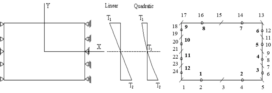
Example 1. Beam Subjected to Linear and

Quadratic Temperature Change

A beam

fixed at both ends is assumed to be subjected to two different cases of temperature change. Plane stress case was assumed and the material of the beam is taken to be, E = 106 _N/m2_{, v = 0.3, α = 10}-7 _deg-1

Figure 1 illustrates the beam geometry and the temperature variation along the depth of the beam. A BEM discretization of the beam is also shown. The numerical solution for the normal stresses, _σx along the y-axis in the center of the beam were compared with analytical solutions. For linear temperature change with T1 = -1000° _{and T2 =}

1000°, the exact values of the normal stress are given analytically by [21],

h y ) T T (

E 1 2

x =− α −

σ

where h is the width of the beam and y is the coordinate shown in Figure 1.

1 2 3 4 5 12 11 10

`9₈ 7 17 16 15 14 13

18 19 20 21 22 23

24 _{1 2} 3

5 6 7 8

9

10

11

12

4

6

For the second case a quadratic temperature variation of the form, T = 2(T1₊T2₋2T3)y2_/h2₊ (T1₋T2)y/h₊T3, with T1 = -20_°, T2 = 40_° and T3 = 0_° is implemented. The exact values for the normal stress under such a temperature distribution are given by [21],

] h y ) T -T ( + h y ) 2T -T + T ( 2 [ E

-= ₂ 1 2

2

3 2 1

x α

σ

The BEM and numerical results can be found in Table 1. As can be seen the accuracy of the numerical formulation is very well satisfied for the two cases of linear and quadratic temperature variation. However, the errors in the case of quadratic temperature variation are slightly higher than the other case, as can be expected.

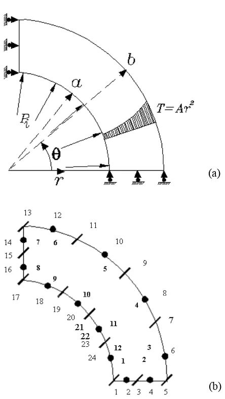
Example 2. Internal Pressure Cylinder Under

Thermal Loading

In this example a cylinder

under combined pressure as well as a temperature gradient is considered. The temperature distribution is assumed to have the form of, T = Ar2_{, where A is}

a constant. The material and geometrical properties are as follows, E=107 N/m2; _α =10-5 deg-1; a = 10cm; b=20cm; Pi=1000 Pa; A=2.5. The answer to this problem is the superposition of the analytical solution from the two cases of loading, i.e., the internal pressure and thermal gradient loading [21]. Figure 2 shows the geometry with temperature distribution and boundary element discretization.

The results are given in Table 2 for radial displacements, radial and tangential stresses. The accuracy of the results is well satisfied

TABLE 1. Normal Stress σσσσx (N/m2) Along The Centerline In Y-Direction For Linear And Quadratic Temperature Distribution In A Beam.

Linear Temperature Distribution Quadratic Temperature Distribution

Y-axes Exact BEM (P.I.) Exact BEM (P.I.)

- 0.500 h - 100.000 -101.2172 - 4.000 -3.9908

- 0.375 h - 75.000 -74.2744 -2.8125 -2.6733

- 0.250 h - 50.000 -51.3937 -1.7500 -1.8046

- 0.125 h - 25.000 -25.1422 -0.8125 -0.8844

0.000 h 0.000 0.00011 0.0000 0.0092

0.125 h 25.000 25.1421 0.6875 0.7440

0.250 h 50.000 51.3937 1.2500 1.2790

0.375 h 75.000 74.2743 1.6875 1.6031

0.500 h 100.000 101.2172 2.0000 1.9935

Figure 2. A pressurized cylinder under a quadratic temperature distribution, (a) Geometry and temperature distribution, (b) BEM discretization. E = 107 _N/m2_.

(b)

TABLE 2. Radial Displacements (cm) And Stresses (N/m2_{) In Axisymmetric Thermoelastic Response For A Pressurized}

Cylinder Under A Radial Temperature Distribution.

Radial Displacement (ur) Radial stress (σσσσr) Hoop stress (σσσσθθθθ)

NODE Exact BEM Exact BEM Exact BEM

1 0.08322 0.08309 -1000.0 -1030.2 27536.12 27554.02

2 0.09051 0.09035 7415.8 7677.17 26833.67 26907.55

3 0.10645 0.10636 8422.72 8413.04 1373.926 1379.19

4 0.13076 0.13053 5737.16 5773.81 -24961.29 -25151.86

5 0.16383 0.16357 0.0 -4.13 -52633.03 -52655.22

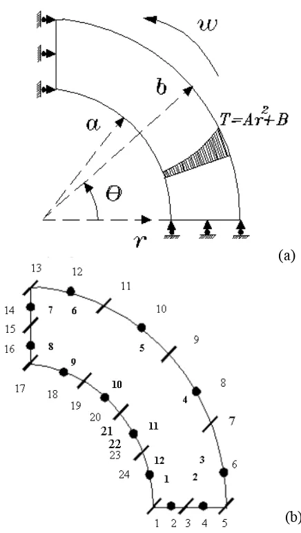
Example 3. Thermal Analysis of Rotating

Disc

Let’s consider a thin disc of uniform

thickness with a central hole, rotating with a constant angular velocity _ω rad/sec and in addition is subjected to a thermal loading according to, T=A r2 + B, where A and B are constants. The analytic solutions for resulting stresses and radial displacement are the superposition of two different cases thermal and inertial loading due to rotation [21].

The appropriate boundary conditions of traction-free edges on a disc with a concentric hole are

σ

r = 0,

at r = a and r = b, the inner and outer radii respectively.

For a plane stress case, the disc has a uniform thickness with inner and outer radii of 0.1m and 0.2 m, respectively. The mesh contains 12 three-node continuous elements and a total of 24 nodes. Because of symmetry, one-fourth of the geometry was modeled as shown in Figure 3. The data used was, E=105 Nm-2; _ν = 0.3; _α = 0.001 deg-1_{; ρ = 2.4 kg/m}3_{; ω = 100 rad/sec; A =}

2500; B = 500.

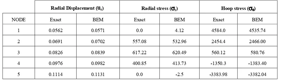
Table 3 contains a comparison between analytical and BEM numerical results using particular integrals for ur and also _σr and _σθ along the radius of the disc. Good agreement is seen for both displacements and stresses due to thermoelastic behavior.

8. ACKNOWLEDGMENT

The first author would like to appreciate the

Figure 3. A rotating disc with temp. distribution T=Ar2_{+B, (a)} Geometry and temperature distribution, (b) BEM model. E = 107 _N/m2_.

(a)

supports provide by the Surface Effect Research Institute at Shiraz during the course of this work.

9. REFERENCES

1. Cruse, T. A., “Numerical Solutions in Three-Dimensional Elastoestatics”, Int. J. Solids and Structs, 5, (1979), 1259-1274.

2. Danson, D. J., “Boundary Element Formulation for Problems in Linear Isotropic Elasticity with Body Forces”, Springer Verlag, 1981.

3. Rizzo, F. J. and Shippy, D. J., “An Advanced B.I.E.M. for Three-Dimensional Thermoelasticity”, Int. J. Num. Meth. Engng., 11, (1977), 1753-1766.

4. Karami, G. and Fenner R. T., “A Two-Dimensional BEM for Thermoelastic Body Force Contact Problems”, in Boundary Elements IX, Vol. 2 Stress Analysis, Editors: C.A. Brebbia, W.L. Wendland, and G. Kuhn, Springer Verlag, Berlin, (1987).

5. Karami, G. and Kuhn G., “Implementation of Thermoelastic Forces in Boundary Element Analysis of Elastic Contact and Fracture Mechanics Problems”, Eng. Anal. with Boundary Elements, 10, (1992), 313-322.

6. Karami, G., “A Boundary Element Method for Two-Dimensional Contact Problems”, Springer-Verlag, Berlin, (1988).

7. Nardini, D. and Brebbia C. A., “A New Approach to Free Vibration Analysis Using BE in BEM”, Springer Verlag, (1982).

8. Wrobel, L. C., “The Dual Reciprocity BE Formulation for Transient Heat Conduction”, Springer Verlag, (1986). 9. Nowak, A. J. and Brebbia, C. A., “The Multiple

Reciprocity Method”, Eng. Anal. with Boundary Elements, 6, (1989), 164-168.

10. Neves, A. C. and Brebbia, C. A., “The Multiple Reciprocity BEM in Elasticity”, Int. J. Num. Meth. Engng., 31, (1991), 709-727.

11. Kuhn, G., “BE Technique in Elastostatics and Linear Fracture Mechanics”, Springer Verlag, (1988), 109-169. 12. Sharp, S. and Crouch, S. L., “Boundary Integral Method

for Thermoelasticity Problems”, J. Appl. Mech. ASME, 53, (1986), 298-302.

13. Watson, J. O.,”Advanced Implementation of the BEM for Two and Three-Dimensional Elastostatics”, Applied Science Publishers, Barking, U.K., (1979), 31-64.

14. Banerjee, P. K. and Butterfield, R., BEM in Engineering Science, McGraw-Hill, London, (1981).

15. Banerjee, P. K. and Ahmad, S., “Free Vibration Analysis by BEM Using Particular Integrals”, J. Eng. Mech. Div. ASCE., 112, (1986), 682-695.

16. Wang, H. C. and Banerjee P. K., “Axisymmetric Free Vibration Analysis by the BEM”, J. Appl. Mech. ASME, 55, (1987), 437-444.

17. Banerjee, P. K., Ahmad, S. and Wang, H. C., “A New BEM Formulation for Acoustic Eigenfrequency Analysis”,

Int. J. Numer. Meth. Engng., 116, (1991), 623-631. 18. Banerjee, P. K. and Wilson, R. B., “Advanced Elastic and

Inelastic Three-Dimensional Analysis of Gas Turbine Engine Structures by BEM”, Int. J. Num. Meth. Eng., 26, (1988), 393-411.

19. Henry, D. P. and Banerjee, P. K., “A New Boundary Element Formulation for Two and Three Dimensional Thermoelasticity Using Particular Integral”, Int. J. Num. Meth. Engng., 26, (1988), 2061-2077.

20. Brebbia, C. A. and Domingues, J., “Boundary Elements: A Course for Engineers”, Computational Mechanics Publications, Southampton, McGraw Hill, New York, (1989).

21. Timoshenko, S. P., “Theory of Elasticity”, McGraw-Hill, London, (1977).

TABLE 3. Radial Displacements (cm) And Stresses (N/m2) In Thermoelastic Response For A Rotating Disc Under A Radial

Temperature Distribution.

Radial Displacement (ur) Radial stress (σσσσr) Hoop stress (σσσσθθθθ)

NODE Exact BEM Exact BEM Exact BEM

1 0.0562 0.0571 0.0 4.12 4584.0 4535.74

2 0.0691 0.0702 557.08 532.96 2454.4 2466.00

3 0.0826 0.0839 617.22 620.49 560.12 580.76

4 0.0976 0.0982 400.85 413.73 -1350.3 -1383.40