Automatic Brain Tumor Segmentation by Deep Convolutional Networks and Graph Cuts

(1)

Western University Western University

Scholarship@Western

Electronic Thesis and Dissertation Repository

1-19-2018 10:30 AM

Automatic Brain Tumor Segmentation by Deep Convolutional

Networks and Graph Cuts

Zhenyi Wang

The University of Western Ontario Supervisor

Veksler, Olga

The University of Western Ontario Graduate Program in Computer Science

A thesis submitted in partial fulfillment of the requirements for the degree in Master of Science © Zhenyi Wang 2018

Follow this and additional works at: https://ir.lib.uwo.ca/etd

Part of the Bioimaging and Biomedical Optics Commons

Recommended Citation Recommended Citation

Wang, Zhenyi, "Automatic Brain Tumor Segmentation by Deep Convolutional Networks and Graph Cuts" (2018). Electronic Thesis and Dissertation Repository. 5189.

https://ir.lib.uwo.ca/etd/5189

This Dissertation/Thesis is brought to you for free and open access by Scholarship@Western. It has been accepted for inclusion in Electronic Thesis and Dissertation Repository by an authorized administrator of

(2)

Abstract

Brain tumor segmentation in magnetic resonance imaging (MRI) is helpful for diagnostics, growth rate prediction, tumor volume measurements and treatment planning of brain tumor. The difficulties for brain tumor segmentation are mainly due to high variation of brain tumors in size, shape, regularity, location, and their heterogeneous appearance (e.g., contrast, intensity and texture variation for different tumors). Due to recent advances in deep convolutional neural networks for semantic image segmentation, automatic brain tumor segmentation is a promising research direction.

This thesis investigates automatic brain tumor segmentation by combining deep convolu-tional neural network with regularization by a graph cut. We investigate several deep con-volutional network structures that have been successful in semantic and medical image seg-mentation. Since the tumor pixels account for a very small portion in the whole brain slice, segmenting the tumor from the background is a highly imbalanced dense prediction task. We use a loss function that takes the imbalance of the training data into consideration. In the sec-ond part of the thesis, we improve the segmentation results of a deep neural network by using optimization framework with graph cuts. The graph cut framework can improve segmentation boundaries by making them more smooth and regular. The main issue when using the segmen-tation results of convolutional neural networks for the graph cut optimization framework is to convert tumor probabilities learned by a convolutional network into data terms. We investigate several possible ways that take into consideration the segmentation artifacts by convolutional neural networks.

In experiments, we present the segmentation results by different deep convolutional neural network structures, e.g., fully convolutional neural network, dilated residual network and U-Net. Also, we compare the combination of U-Net with different data terms for graph cut regularization to improve the neural network segmentation results. Experimental results show that the U-Net performs best with the intersection over union (IoU) for tumors of 0.7286. The IoU for tumors is improved to 0.7530 by training on three slices. Also, the IoU for tumors is improved to 0.7713 by U-Net with balanced loss function. The IoU for tumors is further improved to 0.8078 by graph cut regularization.

Keywords:Automatic brain tumor segmentation, deep convolutional neural network, dense prediction, graph cut regularization.

(3)

Acknowledgement

First of all, I would like to express my sincere gratitude to my supervisor Prof. Olga Veksler who is a great and very nice advisor and inspires me to apply deep learning model to solve computer vision problems. I really appreciate her patience when discussing the next step research directions and looking through the experimental results. And every time when we get stuck she can always come up with new ideas to help us move forward. Her attitude and dedication to work and research encouraged me to do research carefully.

Second, I want to appreciate those helped me with my study and thesis. I am so grateful to work with Dr. Lena Gorelick who helped me to incorporate the deep convolutional neural network output into the energy minimization framework. And I would also like to thank Prof. Yuri Boykov, who has great passion about computer vision and presented very detailed and intuitive explanation in class. His passion and teaching style enabled me to think actively about computer vision research problems and made me realize that computer vision is so interesting. Next, I would like to thank other members in our vision group. I want to give special thanks to Danfeng Chen who did the prior work of this thesis. She always patiently answers my question about previous research work. Thanks all my other friends as well, they bring much fun to my life. Last but not the least, I want to thank my family, especially my great parents and sister, for continuously encourage me to solve problems, support and sincere love.

(4)

List of Figures

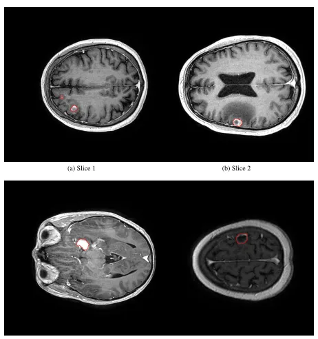
1.1 Slices of brain image. The red contours are the boundaries of the ground truth. The pixels inside the red contour are tumor pixels and the pixels outside the red contour are background pixels. . . 2

1.2 Tumor size is too small. The red contours are the boundaries of the ground truth. The pixels inside the red contour are tumor pixels and the pixels outside the red contours are background pixels. . . 3

1.3 Volume resolution is too small. The red contours are the boundaries of the ground truth. The pixels inside the red contours are tumor pixels and the pixels outside the red contours are background pixels. . . 4

1.4 Volume is too dark. The left volume is too dark and the right volume looks incomplete. These two kinds of volumes are very different from other volumes. 4

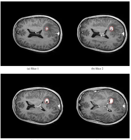
1.5 Examples of brain tumor diversity in size, location and shape. The red contours are the boundaries of the ground truth. The pixels inside the red contours are tumor pixels and the pixels outside the red contours are background pixels. . . . 6

1.6 Examples of inconsistent appearance of tumor. The red contours are the bound-aries of the ground truth. The pixels inside the red contour are tumor pixels and the pixels outside the red contours are background pixels. . . 7

1.7 Examples of similarity between tumor and healthy tissues. The red contours are the boundaries of the ground truth. The pixels inside the red contours are tumor pixels and the pixels outside the red contours are background pixels. . . . 8

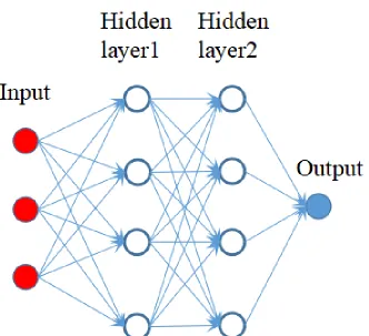
2.1 Examples of fully connected neural networks. The red, white and blue cir-cles are the input, hidden and output units for the neural network. The arrows indicates the connection relationship between neuron units. . . 16

2.2 Examples of convolutional networks by applying a series of filters with size smaller than the input size. Each thin cuboid is one feature channel and is the convolution output of one filter applied on the previous input. . . 17

(8)

2.3 Examples of convolution operations. The above row is obtained by convolution with kernel size 3 applying to the bottom row. The arrows indicate which input units affect which output units. The blue circles in the bottom row affect the outputy3 and are called as the receptive field ofy3. Other units in the bottom row do not have influence on the output units. Eachxiis the input unit andyiis

the output unit. Image is from [15]. . . 17

2.4 Examples of fully connected neural networks. The above row is formed by matrix multiplication with fully connectivity. The arrows indicate which input units affect which output units. All the units with blue circles in the bottom row affect the outputy3. Each xiis the input unit andyi is the output unit. Image is from [15]. . . 18

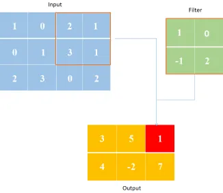
2.5 An example of 2-D convolution with a 2 by 2 filter without kernel-flipping to the input and obtain output. The red square output is the dot product between the square input and the filter. . . 19

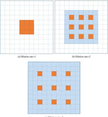
2.6 Examples of convolutions with different dilation rates. The orange squares are the locations where the convolution operates and the blue squares are the locations which are filled with zeros and have no effects on the output. The number of parameters associated with each layer is identical. The receptive field of output units are increased by using larger dilation factors. . . 21

2.7 Applying 2 by 2 max pooling to the left activation map and obtain the right output. . . 22

2.8 T-links weights for a pixel pin the graph . . . 29

2.9 6-neighborhood system. Each voxel has four connections to its immediate left, right, top, bottom neighboring pixels within the same slice, and two connec-tions to its closest neighbor pixels in the previous and next slice. . . 30

2.10 An s−tcut on graph with two terminals. [Image credit: Yuri Boykov] . . . 31

2.11 Binary segmentation for 3×3 image. (top-left): Original image; (top-right): Graph constructed based on original image with extra s and t terminals; (bottom-right) A minimal cut for the graph separating all pixels into two disjoint sets; (bottom left): Segmentation result, one color stands for one label. [Image cred-it: Yuri Boykov] . . . 33

3.1 Examples of overlapping crops. The boxes with different colors are the corre-sponding crops on the original image. . . 37

3.2 Modified fully convolutional neural network architecture . . . 39

3.3 Modified U-Net architecture . . . 40

3.4 Residual learning: a building block. . . 41

(9)

3.5 Dilated residual networks architecture. Each rectangle is a Convolution-Batch normalization-Relu activation group and the numbers mean the number of fil-ters in that layer. The red connection besides the rectangle is the skip con-nection. And the number between two blue lines is the dilation rate for the corresponding convolutional layers. . . 42 3.6 Visualization of data term (e). The vertical and horizontal lines in (b) and (c)

are the crop boundary. . . 49 3.7 Visualization of data term (f). . . 50

4.1 Examples of intersection over union, which is calculated by the intersection, indicated by the blue area, divided by the union of the two rectangle. . . 53 4.2 Segmentation results of part of one volume using only FCN. The red contour

is the boundary of the ground truth, and the yellow contour is the boundary of the segmentation. . . 55 4.3 Segmentation results of part of one volume using only FCN. The red contour

is the boundary of the ground truth, and the yellow contour is the boundary of the segmentation. . . 56 4.4 Segmentation results of part of one volume using only FCN. The red contour

is the boundary of the ground truth, and the yellow contour is the boundary of the segmentation. . . 57

4.5 Segmentation results of part of one volume using only U-Net. The red contour is the boundary of ground truth, and the yellow contour is the boundary of the segmentation. . . 58 4.6 Segmentation results of part of one volume using only U-Net. The red contour

is the boundary of ground truth, and the yellow contour is the boundary of the segmentation. . . 59 4.7 Segmentation results of part of one volume using only U-Net. The red contour

is the boundary of ground truth, and the yellow contour is the boundary of the segmentation. . . 60 4.8 Segmentation results of part of one volume using only DRN. The red contour

is the boundary of ground truth, and the yellow contour is the boundary of the segmentation. . . 61

4.9 Segmentation results of part of one volume using only DRN. The red contour is the boundary of ground truth, and the yellow contour is the boundary of the segmentation. . . 62 4.10 Segmentation results of part of one volume using only DRN. The red contour

is the boundary of ground truth, and the yellow contour is the boundary of the segmentation. . . 63

(10)

4.11 Comparison of segmentation results using only one slice and 3 slices. For each row, the left image is the segmentation result using only one slice and the right image is the segmentation result using 3 slices. The red contour is the ground truth boundary, and the yellow contour is the segmentation boundary by U-Net. 64

4.14 Comparison of segmentation results using balanced loss function whenβ=0.15 andβ=0.5. For each row, the left image is the segmentation result usingβ=0.15 and the right image is the segmentation result usingβ=0.5. The red contour is the ground truth boundary, and the yellow contour is the segmentation bound-ary by U-Net. . . 67

4.17 Comparison of segmentation results using only Net and combination of U-Net with graph cut regularization. For each row, the right image is the segmen-tation using only U-Net and the left image is the segmensegmen-tation using U-Net and graph cut regularization. The red contour is the ground truth boundary, the blue contour is the segmentation boundary by combing U-Net with graph cut regularization, and the yellow contour is the segmentation boundary by U-Net. . 71

(11)

4.18 Comparison of segmentation results using only Net and combination of U-Net with graph cut regularization. For each row, the right image is the seg-mentation result using only U-Net and the left image is the segseg-mentation re-sult using U-Net and graph cut regularization. The red contour is the ground truth boundary, the blue contour is the segmentation boundary by combing U-Net with graph cut regularization, and the yellow contour is the segmentation boundary by U-Net. . . 72 4.19 Comparison of segmentation results using only Net and combination of

U-Net with graph cut regularization. For each row, the right image is the seg-mentation result using only U-Net and the left image is the segseg-mentation re-sult using U-Net and graph cut regularization. The red contour is the ground truth boundary, the blue contour is the segmentation boundary by combing U-Net with graph cut regularization, and the yellow contour is the segmentation boundary by U-Net. . . 73 4.19 Comparison of segmentation results using only Net and combination of

U-Net with graph cut regularization. For each row, the right image is the seg-mentation result using only U-Net and the left image is the segseg-mentation re-sult using U-Net and graph cut regularization. The red contour is the ground truth boundary, the blue contour is the segmentation boundary by combing U-Net with graph cut regularization, and the yellow contour is the segmentation boundary by U-Net. . . 74

(12)

List of Tables

4.1 Evaluation metrics for the segmentation performance of different deep convo-lutional neural networks. . . 54 4.2 Evaluation metrics for the performance of training on single and three slices . . 64 4.3 Evaluation metrics with different balance weight for the balanced loss function . 69 4.4 IoU of combining U-Net with graph cut regularization. . . 70 4.5 Performance evaluation by setting different threshold for data term f. . . 70 4.6 Evaluation metrics for the performance of training on smaller crops and larger

crops . . . 74

(13)

List of Appendices

(14)

Chapter 1 Introduction

Brain tumors can be classified into two types: cancerous tumors and benign tumors. Magnetic resonance imaging (MRI) provides detailed images of the brain, and is one of the most com-mon ways used to diagnose brain tumors. Brain tumor segmentation from MRI is helpful for improved diagnostics, growth rate prediction and treatment planning for brain tumors and is crucial for monitoring tumor growth or shrinkage in patients during therapy. Also, it is impor-tant in surgical planning or radiotherapy planning. In these cases, the tumor has to be outlined and surrounding healthy tissues are also of interest for further treatment and processing.

Fast and accurate segmentation of a brain tumor is a non-trivial task. The difficulties for brain tumor segmentation are mainly due to high variation of brain tumors in size, shape, regularity, location, and their heterogeneous appearance (e.g., contrast, intensity and texture variation for different tumors).

Previous brain tumor segmentation approaches can be classified into two categories: in-teractive segmentation [35, 9, 29, 17, 19] and automatic segmentation [16, 62, 53, 1, 25, 40, 47, 2, 8]. Interactive segmentation does not rely on a large training data set. It requires user input, e.g., specifying object of interest or adding seeds indicating the labels of some pixels to belong to certain class. The interactive segmentation also allows users to evaluate the result. Then, users edit and refine the results by adding more seeds if the segmentation results are not satisfactory. Interactive segmentation process can be repeated until no further modification is needed. Although interactive segmentation can obtain good segmentation results, trained experts still need to put much effort into performing segmentation until they get satisfactory re-sults. Hence, this thesis aims to investigate automatic brain tumor segmentation by combining deep convolutional neural networks with graph cut regularization to help automatically obtain tumor segmentations.

This thesis utilizes a previously successful interactive brain segmentation system [35, 9], but does not require users to provide input. This thesis shows how to segment the tumor for the whole slice automatically.

(15)

2 Chapter1. Introduction

1.1 MRI and Brain Tumor

This thesis uses MRI-based image data. A magnetic resonance imaging (MRI) scan is a ra-diology technique that uses magnetism, radio waves, and computers to form pictures of the anatomy and the physiological processes of the body in both healthy and non-healthy tissues [11]. MRI can provide a very detailed description of organs and detect tiny body structure changes of the human body. Detailed MRI allows physicians to evaluate various body parts and determine whether certain diseases are present or not.

(a) Slice 1 (b) Slice 2

Figure 1.1: Slices of brain image. The red contours are the boundaries of the ground truth. The pixels inside the red contour are tumor pixels and the pixels outside the red contour are background pixels.

(16)

1.1. MRIandBrainTumor 3

many factors, including imaging parameters, magnet strength, the time allowed for acquisition, etc.

Our data is provided by Aaron Ward and Glenn Bauman from Lawson Health Research Institute. There are 64 MRI brain scans from 27 patients. Some scans are from the same patient in different stages. Each volume has a ground truth, where each pixel is labeled as tumor or background, provided by Glenn Bauman, who is a radiation oncologist and London Regional Cancer Program Professor. Some ground truth is imprecise because it was obtained by blob-manipulation tools. We remove some volumes. Then, we have 45 volumes. Some volumes are deleted for several reasons. First, tumors in some volumes are too small. If we add these volumes into training set, it will cause neural network to fit these small tumors. When making predictions on test data, the neural network will generate false positives. Second, the slice resolution of some brain volumes is too small compared to that of other brain volumes. Significantly resizing these volumes to larger size will change original information. Third, some volumes are too dark and different from most of other volumes. Finally, some volumes do not have voxels that are labeled as tumors. Figures 1.2, 1.3 and 1.4 show some examples of removed volumes.

(17)

(a) Slice 1 (b) Slice 2 (c) Slice 3 (d) Slice 4

Figure 1.3: Volume resolution is too small. The red contours are the boundaries of the ground truth. The pixels inside the red contours are tumor pixels and the pixels outside the red contours are background pixels.

Figure 1.4: Volume is too dark. The left volume is too dark and the right volume looks incom-plete. These two kinds of volumes are very different from other volumes.

(18)

1.2. Challenge forBrainTumorSegmentation 5

large enough because deep neural networks usually have lots of parameters to be learned and small size of training data will be very likely to cause overfitting. And tumor shape, location, size and appearance cases should be as diverse as possible in training data since to make the neural networks generalize better, we should enable neural networks to see lots of different training examples. The test set could be larger but, if the test set is larger, we will have less training and validation data, which will not be enough for neural networks to learn a good mod-el. We adopt simple data augmentation only on training and validation data, i.e., horizontal and vertical flipping of the image crops. We add these augmented data into the whole training and validation data, tripling the number of training and validation images. No other data augmen-tation is used. Thus, by data augmenaugmen-tation, the training set contains 27294 image crops and the validation set contains 7050 image crops. The crop size is 128× 128 pixels. The voxels are represented by 16-bit integers. The Multimodal Brain Tumor Image Segmentation Benchmark (BRATS) challenge is organized in conjunction with the international conference on Medical Image Computing and Computer Assisted Interventions (MICCAI). Also, our dataset is diff er-ent from BRATS dataset [42] and we only have tumor and healthy brain tissue, i.e., a binary classification problem. Annotations of BRATS dataset comprise the GD-enhancing tumor, the peritumoral edema, the necrotic and non-enhancing tumor, as described in [42].

1.2 Challenge for Brain Tumor Segmentation

(19)

(c) Slice 3 (d) Slice 4

(20)

1.2. Challenge forBrainTumorSegmentation 7

(21)

Figure 1.7: Examples of similarity between tumor and healthy tissues. The red contours are the boundaries of the ground truth. The pixels inside the red contours are tumor pixels and the pixels outside the red contours are background pixels.

Diversity in Size, Location and Shape

(22)

1.3. Overview ofMRI-basedBrainTumorSegmentation 9

shape, we can observe its diversity in 2D slice images. The diversity of size, location and shape in brain tumors obstructs automatic segmentation to obtain satisfactory results. Figure 1.5 shows different size, location and shape of different tumors.

Highly Imbalanced Tumor over Background

Since the tumor area only accounts for a small area of the whole slice image in our dataset, usually less than 1%, segmenting tumors from background is a highly imbalanced dense pre-diction task, as indicated in Figure 1.1. When applying machine learning model to perform automatic segmentation, we should pay attention to dealing with this issue.

Inconsistency in Appearance

Different parts of one tumor may have different appearance even if they belong to the same connected component. For different slices of brain tumors, they usually have very different appearance. Figure 1.6 shows several examples with inconsistent tumor appearance. This adds to the difficulty of methods based on appearance models. Also, when applying machine learning approaches, the features extracted should capture these kinds of appearance variance.

Similarity between tumor and healthy tissue

Sometimes, surrounding healthy tissues are very similar to tumors. In this case, appearance is similar between the tumor and the background. If strong contrast boundaries exist between the tumor and healthy tissue, one can still segment the tumor by utilizing the intensity contrast information. Otherwise, it is difficult to locate tumor for an untrained human. In many cases, a tumor could be very similar to some other brain parts, as illustrated in Figure 1.7. This kind of tissues often further increase the difficulty of the segmentation process. When applying machine learning model, it will be hard to discriminate tumor from background and predict the labels correctly.

1.3 Overview of MRI-based Brain Tumor Segmentation

There are various existing interactive brain tumor segmentation approaches. An interactive brain tumor segmentation method using graph cuts is presented in [5]. 3D Slicer is used as an interactive tool for brain tumor segmentation [29]. A k-nearest neighbors algorithm based method [17] uses some minimum user interaction to segment a given brain by training and generalizing within that brain only. A Bayesian inference based interactive 3D brain segmen-tation is in [19], where user inputs are formulated as a probabilistic spatial term in a level set functional.

(23)

results. In the preprocessing stage, certain image enhancement techniques, such as image de-noising, intensity normalization and skullstripping, can be used for improving image quality. For enhanced images, commonly used image features, e.g., image intensity, local image tex-ture, gradient features can be either extracted from one single modality or from multi-modal images. Various features from MRI can be used alone or combined together for automatic brain tumor segmentation.

Automatic segmentation algorithms can be categorized into classification and clustering methods according to whether they apply machine learning models in a supervised or an unsu-pervised way. First, these methods extract feature vectors, e.g., texture features, from voxelwise intensity. Then, the extracted feature vector is used as input to the machine learning model to decide for every voxel which class it belongs to. However, simple voxelwise classification or clustering methods do not make use of complete image information. Therefore, additional constraints, e.g., neighborhood regularization, shape and localization constraints are added in-to some methods. A random field regularization method is often imposed inin-to neighborhood constraints, while deformable models can be used for shape constraints [4].

Clustering models work in an unsupervised way and cluster voxels into several groups based on certain similarity metrics [55]. On the other hand, other approaches for brain tumor segmentation employ classification models. Classification models require training data to learn a classification model using handcrafted features and ground truth annotations. Unlike cluster-ing approaches, these approaches utilize little prior information on the brain structure, but they need to extract high dimensional low level image features. Then, using classification method directly models the relationship between these features and the label of a given voxel. These features could be raw input voxel intensity values [17] , local intensity histogram [41] and texture features such as Gabor filterbanks [51]. Classical discriminative learning techniques such as support vector machine [3] and decision and random forests [61, 14, 42] have also been applied to classify each voxel to be a certain tumor class.

(24)

1.4. ConvolutionalNeuralNetworkApproach forBrainTumorSegmentation 11

1.4 Convolutional Neural Network Approach for Brain

Tu-mor Segmentation

Previous automatic brain tumor segmentation approaches depend on hand-engineered features that exploit very generic edge-related information for general computer vision tasks, but with-out specific adaptation to the domain of brain tumors. For automatic brain tumor segmentation, one would like to use features that are composed and refined into the domain of brain images. By utilizing these better features, the machine learning models are expected to be able to better segment the tumor from the background. Recently, deep convolutional neural networks (C-NNs) have been successful in various computer vision tasks [49, 18, 36, 57, 10, 44, 13, 45] and can learn hierarchical features that are useful for various tasks. Preliminary investigations have demonstrated that applying deep CNNs for automatic brain tumor segmentation is a very promising approach [16, 62, 53].

Some previous methods first divide the 3D MR images into 2D or 3D patches. Then, a deep CNN is trained to predict the label of its center voxel. Urban et al. [53] and Zikic et al. [62] implemented a common deep CNN architecture, which consists of a series of convolutional layers and a non-linear activation function between each consecutive layer. And a final soft-max output layer is used for calculating the probability of being each class. Havaei et al. [16] proposed a two-pathway CNN architecture that learns about the local brain structure informa-tion as well as larger context informainforma-tion. Obviously, these strategies [16, 62, 53] have two drawbacks. First, they are not efficient because the deep networks must be run independently for each patch, and there is a lot of redundancy when predicting the labels of nearby pixels due to overlapping patches between neighbouring pixels. Since these approaches are patch-based and once forward propagation can only predict one pixel label, they are very slow compared to dense prediction based approaches, which predict all pixel labels in one whole image by once forward computation [36, 57, 46]. Secondly, there is a trade-offbetween computational cost and the use of context. Larger patches require more computation, but can utilize more context information; while small patches allow the network to only see small context, but computation cost is low.

(25)

subsam-12 Chapter1. Introduction

pling layers that reduce resolution to obtain a global prediction. In contrast, dense prediction for semantic image segmentation requires full-resolution output. Fully convolutional neural networks have been used for brain tumor segmentation [1, 25, 40, 47]. Dilated convolutional networks have been used for semantic segmentation by multi-scale context aggregation [57] and have been applied for brain tumor segmentation [34, 37, 60]. U-Net based convolutional network [46] has been used for biomedical image segmentation. Also, 3D U-Net [2, 8] is adopted for brain tumor segmentation.

1.5 Our Approach

The goal of this thesis is to evaluate the network architectures that have been successful in semantic image segmentation and brain segmentation to find the architecture that works best for our data. In addition, we use graph cut optimization to further improve the segmentation results by regularizing the segmentation boundary obtained from a neural network.

Since the tumor area only accounts for a small proportion of the whole brain slice in our dataset, usually less than 1%, segmenting tumors from background is a highly imbalanced dense prediction task. To deal with this issue, we crop the whole slice image into overlapping crops. Also, by doing this, we can speed up the training process compared to training on the whole slice. First, we train the deep convolutional neural network, including fully convolution-al neurconvolution-al network [36], dilated residuconvolution-al network [57] and U-Net [46], to segment each crop of whole slices. Then, we combine the segmentation results of all crops together by a simple union operation when testing on test slice image. We consider performing the segmentation slice by slice from the axial view. Thus, the deep CNNs sequentially process each 2D slice.

Then, we apply graph cut optimization to further refine the neural network segmentation results. When we use energy minimization framework to perform segmentation, the two com-monly used energy terms are the data term and smoothness term. Data term, also called re-gional term, contains rere-gional appearance information. Smoothness term, or boundary term, encodes the coherence information among image pixels. Three deep convolutional neural net-works adopted in this thesis take the image as input and output a probability map for each class and each pixel. Then, we convert these probabilities into different data terms and incorporate them into the graph cut energy minimization framework.

To reduce the shrinking effect of the graph cut algorithm, we introduce a ballooning bias as in [9]. Volume ballooning adds ballooning bias to the energy function so that the pixel can get a bonus if it is assigned to the foreground. Volume ballooning is encoded as an unary term in energy function and can be easily integrated into the energy optimization framework.

The main contributions we have are as following:

(26)

1.6. Outline ofThisThesis 13

automatic brain tumor segmentation.

2. We evaluate previous successful fully convolutional networks to perform brain tumor segmentation.

3. We combine deep CNNs with graph cut regularization and use different data terms to improve the deep neural network segmentation results.

We optimize all the parameters of the graph cut segmentation by grid search on the valida-tion data and use these parameters on test data.

1.6 Outline of This Thesis

(27)

Chapter 2 Related Work

2.1 Deep Convolutional Neural Network

Deep learning [15] has been successful in computer vision, natural language processing and speech recognition. Convolutional networks [32], also known as convolutional neural networks (CNNs), are a special kind of neural network for processing data that has grid-like topology, e.g., image data, which can be thought of as a 2D grid of pixels. CNNs have achieved the state-of-the-art performance in various computer vision applications, including image recognition [49, 18], semantic segmentation [36, 57, 10, 44], object detection [13, 45], stereo matching [59], etc. Convolutional neural networks use a linear operation called convolution and are simply neural networks that use convolution in place of general matrix multiplication in at least one of their layers.

Convolutional networks were inspired by biological processes [22, 20, 21] in which the connectivity relationship between neurons is inspired by the anatomy structure of the animal visual cortex. Individual cortical neurons only respond to stimuli around a restricted area of vi-sual field, also known as the receptive field. The receptive fields of different neurons partially overlap with each other such that these neurons cover the whole visual field. Neurophysi-ologists David Hubel and Torsten Wiesel collaborated for several years with neuroscientific experiments to explore and discover how the mammalian vision system works [22, 20, 21]. Their great discovery was that neurons in visual system responded very strongly to specific patterns of light, but they almost did not respond at all to other light patterns. These discover-ies were long before the relevant computational convolutional network models were developed and have had great influence on contemporary deep learning models.

Convolutional neural networks are very similar to ordinary neural networks and are made up of neurons that have learnable weights and biases. Each neuron receives some inputs, per-forms a dot product operation and optionally follows it with a non-linearity activation function. The entire neural network still represents a single differentiable function, i.e., from the raw

(28)

2.1. DeepConvolutionalNeuralNetwork 15

put image pixels on one end to class scores at the other. Also, they still have a loss function (e.g. cross entropy) on the last layer. All the approaches that are developed for learning gen-eral neural networks parameters still apply to CNNs. CNN architectures make the explicit assumption that the inputs of the networks are images, which allows us to incorporate certain properties into the architecture.

Convolutional neural networks leverage three important ideas that can help improve a ma-chine learning system, i.e., sparse interactions, parameter sharing and equivariant representa-tions [15], which will make the forward function more efficient to be implemented and dramat-ically reduce the amount of parameters in the whole network. Also, convolution provides ways for dealing with inputs of variable size.

For traditional neural network layers, every output unit interacts with every input unit, as shown in Figure 2.1. However, convolutional neural networks typically have sparse interac-tions between input and output units, also referred to as sparse connectivity, which is achieved by setting the kernel size of CNNs smaller than the input size, as shown in Figure 2.2. For ex-ample, when processing an image, the input image might have thousands or millions of pixels, but we can still extract meaningful features, e.g., edges features, with kernels that only occupy a small and restricted area. There are several benefits by doing this. First, we only need to store fewer parameters, which reduces the memory requirements of the model. Figures 2.3 and 2.4 show the difference of the connectivity and parameters needed in convolutional net-work and fully connected netnet-work. They also show the receptive field difference of one unit in convolutional network and fully connected network. Second, it also means that computing the output usually requires much fewer numerical computation. These improvements in efficiency are often quite significant in real applications.

Parameter sharing refers to using the same parameter for more than one function in a neural network model, i.e., the value of the weight applied to one input is tied to the value of a weight applied elsewhere. In a traditional neural network, each element of the weight matrix is used exactly only once when computing the output of one layer. In a convolutional neural network, each member of the kernel is used at every pixel of the input image (except perhaps some pixels around the image boundary, depending on the design that uses some techniques about how to deal with the boundary pixels, e.g., zero padding around the input image boundary). The parameter sharing adopted by the convolution operation means that rather than learning a separate set of parameters for every location, we only need to learn one set of parameters that are shared by all locations. This will further reduce the memory storage requirements of the model. Thus, convolution operation is vastly more efficient than dense matrix multiplication in terms of memory requirements and the number of parameters to be learned.

(29)

16 Chapter2. RelatedWork

convolution layer creates a 2D map of where certain features appear in the input. If we move the object a bit in the input, the feature representation of the input will also move the same amount in the output.

(30)

Figure 2.2: Examples of convolutional networks by applying a series of filters with size smaller than the input size. Each thin cuboid is one feature channel and is the convolution output of one filter applied on the previous input.

(31)

Figure 2.4: Examples of fully connected neural networks. The above row is formed by matrix multiplication with fully connectivity. The arrows indicate which input units affect which output units. All the units with blue circles in the bottom row affect the outputy3. Each xi is

the input unit andyi is the output unit. Image is from [15].

In this chapter, we describe some operations in deep CNNs that are used in this thesis. We first describe what the convolution operation is. Next, we describe an operation that generalizes convolution operation called dilated convolution. Then, we describe an operation called pool-ing, which almost all convolutional networks employ. Then, we describe batch normalization, which is an useful technique to make it easier for training deep neural networks. Finally, we describe the challenges and optimization algorithms in training neural networks.

2.1.1 Convolution Operation

Usually, the operation used in a convolutional neural network does not correspond precisely to the definition of convolution as used in other fields such as engineering or pure mathematics. We describe several variants on the convolution function that are widely used in practice for neural networks.

In its most general form, convolution is an operation on two functions of a real valued argument. If we use a two-dimensional imageI and a two-dimensional kernelK as the input, the convolution operation is:

(I∗K)(i, j)= X

m X

n

I(m,n)K(i−m, j−n) (2.1) Convolution is commutative, meaning we can equivalently write:

(K∗I)(i, j)= X

m X

n

(32)

Usually the Equation 2.2 is more straightforward to implement in a deep learning library, because there is less variation in the range of valid values ofmandn. The commutative property of convolution arises because we have flipped the kernel relative to the input, in the sense that as

mincreases, the index into the input increases, but the index into the kernel decreases. The only reason to flip the kernel is to obtain the commutative property. Many deep learning libraries implement a related function called the cross-correlation, which is the same as convolution but without flipping the kernel. Figure 2.5 shows an example of convolution operation.

(I∗K)(i, j)= X

m X

n

I(i+m, j+n)K(m,n) (2.3) Equation 2.3 defines the cross-correlation operation.

(33)

2.1.2 Dilated Convolution

LetI :Z2 _→_R_{be a discrete function. Let}Ω

r =[−r,r]2∩Z2andK :Ωr→ Rbe a discrete filter

of size (2r+1)2_{. The discrete convolution operator}_∗_{on input}_I _{and filter}_K _{can be defined as} the following:

(I∗K)(p)= X

s+t=p

I(s)K(t) (2.4)

Let l be a dilation factor which determines the amount of spaces between neighbouring elements of the convolution operation and let operator∗lbe defined as the following:

(I∗lK)(p)= X

s+lt=p

I(s)K(t) (2.5)

The operator ∗l is a generalization of the convolution operator ∗. Dilated convolution is

the convolution operation with filters that have spaces between each element, called dilation. Then, it can be used for increasing the receptive field but without increasing the number of pa-rameters. Figure 2.6 shows three examples of the dilated convolution operation. Operator∗l is

called a dilated convolution or anl-dilated convolution [57]. The familiar discrete convolution ∗ is simply the 1-dilated convolution. The dilated convolution operator has been referred to

in the past as convolution with a dilated filter. It plays a key role in the algorithme `atrous, an algorithm for wavelet decomposition [38, 48].

(34)

(a) Dilation rate=1 (b) Dilation rate=2

(c) Dilation rate=3

(35)

2.1.3 Pooling

A typical convolutional neural network layer consists of three steps. First, the convolutional layers perform several convolutions to produce a set of linear activations. Second, a nonlinear activation function, e.g., the rectified linear activation function and softmax activation function, is applied for each linear activation. In the third step, a pooling function will be used to modify the nonlinear activations further.

A pooling operation computes a summary statistic of the nearby outputs of the previous layer at a certain location. For example, the max pooling operation takes the maximum value within a rectangular neighborhood, as shown in Figure 2.7. Other pooling functions include the average of a rectangular neighborhood, the L2 norm of a rectangular neighborhood, etc. The intuition behind using pooling is that the precise location of a feature is less important than its rough location. The pooling layer can reduce the resolution of the feature representations, the number of parameters and amount of computation. In some sense, it is useful for controlling overfitting. It is common to apply a pooling layer between successive convolutional layers in deep CNNs. A pooling operation makes the feature representations become approximately invariant to small translation. Invariance to translation indicates that if the input is translated by a small amount, most of the pooled values do not change. Invariance to local translation will be useful when some feature is present is more important the exact location.

(36)

2.1.4 Batch Normalization

Batch normalization [24] is an adaptive reparametrization method and is used for solving the difficulty of training very deep models. In practice, it is very useful for making it easier to optimize deep neural networks.

Essentially, very deep models are the composition of many functions. Training very deep networks is complicated because the inputs to each layer are affected by the parameters of all preceding layers, and the parameters of all the layers are updated simultaneously. When we update the parameters, unexpected results can happen, e.g. gradient vanishing and gradient explosion, because many functions or layers composed together are updated simultaneously. In these cases, it will be very difficult to choose an appropriate learning rate, e.g., for stochastic gradient descent, because the effects of updating the parameters of one layer strongly depend on the parameters of all the other layers.

Batch normalization provides a simple and effective way of reparametrizing almost any deep network. The reparametrization of a deep neural network can significantly simplify the problem of coordinating updates across many layers. Batch normalization can be used for any input or hidden layers in a neural network. In the following, we describe how batch normaliza-tion works.

Consider a mini-batchBof sizem. Since the normalization is applied to each activation in-dependently, let us focus on a particular activationx. Thus, we havemvalues of this activation in the mini-batch, which are denoted byB = {x1...m}. The procedure of batch normalization is

shown in the following steps.

First, normalize the batch of values B = {x1...m}using the mean and variance of the batch

calculated as:

µB =

1

m

m X

i=1

xi (2.6)

and σ2 B = 1 m m X

i=1

(xi−µB)2, (2.7)

whereµBis the mini-batch mean andσ2_Bis the mini-batch variance.

Then, calculate the normalized values ˆx1...mas:

ˆ

x1...m=

xi−µB

q

σ2

B+

, (2.8)

(37)

by normalization. Then, we apply linear transformations to the normalized values ˆx1...m:

yi =γxˆi+β. (2.9)

The variables γ and β are learned parameters that allow the new normalized values y1...m

to have any mean and standard deviation. Normalizing the value of a unit can reduce the expressive power of the neural network containing that unit. In order to maintain the expressive power of the network, it is common to replace the batch of hidden unit activations x1...m with

y1...m. The new parametrization can represent the same family of functions of the input as the

old parametrization of the network, but the new parametrization of the network is much easier to be trained with gradient descent.

In convolutional networks, we need to apply the same normalizingµandσat every location in a feature map to ensure that the statistics of the feature map are the same across all the spatial locations [15].

2.1.5 Training the neural networks

Optimization algorithms are important in training deep neural networks because the training process is expensive. Researchers have developed a specialized set of optimization algorithms for solving it.

Training neural networks involves solving one particular case of the optimization problem-s: finding the parameters W of a neural network that minimize a loss function L(W) which typically consists of a performance measure evaluated on the training data and additional reg-ularization terms. Optimization algorithms for training deep neural networks also typically include some special structure of machine learning optimization objective functions.

Difficulties of training deep neural networks

The difficulty of general optimization can be avoided in traditional machine learning model if we carefully design the objective function and constraints so that the optimization problem is convex. However, we must deal with the general non-convex optimization problem when training neural networks. There are several challenges, e.g., ill-conditioning of the Hessian matrix, local minima, saddle points, etc [15], when optimizing the loss function of neural networks.

(38)

and can cause stochastic gradient descent to increase the loss value even with a very small learning rate.

(2) For a convex optimization problem, any local minimum is also a global minimum. Non-convex functions, e.g., the loss function of deep neural networks, can have many local minima. In practice, there will be an exponentially large number of local minima for the loss function of very deep neural networks. Local minima can be problematic if they have high loss values in comparison to the global minimum. If the local minima with high cost are common, the optimization problem will be difficult. But for sufficiently large neural networks, most local minima have low loss function values, and it is often acceptable to find a set of parameters with a low loss function value, but not necessarily global minimum. In this case, local minima are not major problems.

(3) For many high dimensional non-convex functions, local minima (maxima) are rare and saddle points are more common. In many real applications, the number of saddle points is far more than the number of local minima. A saddle point of a function is a stationary point, where its derivative or gradient is zero, but not an extremum. Some points around a saddle point have larger function values than the saddle point, while other points have smaller function values. At a saddle point, the Hessian matrix has both positive and negative eigenvalues. The gradient magnitude around a saddle point is often small. On the other hand, first order methods, including gradient descent, block coordinate descent, etc, almost always escape saddle points [33], but gradient descent may take exponential time to escape saddle points [12].

(4) There may also be wide and flat regions with constant value. In these regions, the gradient as well as the Hessian matrix are all zero. These degenerate cases are major problems for numerical optimization algorithms. For a convex optimization problem, a wide and flat region must consist of all the global minima, but for a general optimization problem, such a region may have a high objective function value.

Optimization algorithms for training neural networks

In this section, we describe some commonly used optimization algorithms, e.g., stochastic gra-dient descent, Nesterov’ s accelerated gragra-dient [43] and Adam [30], for training deep learning models, as described in [26]. Assume the goal is to minimize the loss function. For a dataset

D, the optimization objective function is the average loss over all|D|data instances, as shown in the following:

L(W)= 1 |D|

|D|

X

i

(39)

where fW(Xi) is the loss evaluated on data instance Xi andr(W) is the regularization term

with weightλ. In practice, the data size|D|could be very large, so a stochastic approximation of the objective function, i.e., by drawing a mini-batch with size N from the whole |D|data instances, is adopted:

L(W)≈ 1

N

N X

i

fW(Xi)+λr(W) (2.11)

The model computes fW(Xi) in the forward propagation and the gradient∇fW in back

prop-agation. The parameters update 4W consists of the gradient∇fW and the regularization term

gradient∇rW. In the following section, we describe three commonly used optimization

algo-rithms for training deep neural networks.

(1) Stochastic gradient descent

Stochastic gradient descent (SGD) uses a linear combination of the previous weight update

Vt and the negative gradient ∇L(W) to update the weightsW. The learning rateα is the

weight on the negative gradient∇L(W). The momentum µis the weight on the previous updateVt. SGD computes the updated valuesVt+1and the updated weightsWt+1at iteration

t+1 using current weightsWtand the previous weight updateVtby the following way:

Vt+1= µVt −α∇L(Wt) (2.12)

and

Wt+1 =Wt +Vt+1, (2.13)

whereαandµare the learning hyperparameters.

(2) Nesterov’ s accelerated gradient

Nesterov’ s accelerated gradient (NAG) appears in [43] and achieves a convergence rate of O(1/t2_{) instead of} _O₍₁/_t_{) for convex optimization problems. Because of the} non-smoothness and non-convexity of the loss function of the deep neural networks, the as-sumptions in the NAG algorithms [43] do not hold. In practice, NAG is a very effective method when optimizing certain types of deep neural network architectures [52].

The weight update formulas are:

(40)

2.2. EnergyMinimizationFramework 27

and

Wt+1 =Wt +Vt+1. (2.15)

(3) Adam

The Adam [30] is a gradient-based optimization method and includes an adaptive moment estimation (mt,vt). The update formulas are shown as:

(mt)i =β1(mt−1)i+(1−β1)(∇L(Wt))i (2.16)

and

(vt)i = β2(vt−1)i+(1−β2)(∇L(Wt))2i. (2.17)

Kingma et al. [30] proposed to useβ1 =0.9,β2= 0.999 and =10−8as default parameter values.

2.2 Energy Minimization Framework

In this section, we describe the energy minimization framework and three energy function terms, including data term, smoothness term and volumetric bias term.

2.2.1 Energy Minimization

Image segmentation can be formulated as a labeling problem, where the problem is to assign each pixel p∈Ω, a label fpfrom some finite setL. The goal is to find a labeling f that assigns

each pixel p ∈ P a label fp ∈ L, where f is both piecewise smooth and consistent with the

observed data. Let f=[fp ∈L|∀p ∈ Ω] be the labeling of all pixels. This problem can be

expressed naturally in terms of energy minimization [7]. One formulates the energy function

E(f) that typically consists of unary term Dp(fp) and pairwise term Vpq(fp, fq). A standard

energy function can be formulated as:

E(f)=X

p∈Ω

Dp(fp)+λ X

pq∈N

Vpq(fp, fq). (2.18)

In Equation (2.18),Dp(fp) is called data term, which is the cost when pixel pis assigned to

label fp. Vpq(fp, fq) is the smoothness term, which regularizes segmentation discontinuities. λ

(41)

2.2.2 Data Term

As discussed in Section 2.2.1, the data term measures how well the labeling fit into the observed data and is usually described by the appearance model. In the binary segmentation case, it represents the cost for assigning a pixel p to be object or background. The negative log-likelihood of the image intensity histogram is often used as data term and is also adopted in [35, 9]. The log-likelihood function,logPr, means the log probability of the pixel passigned to the corresponding label. Higher probability means that the pixels are more likely to be assigned to the corresponding label, and thus incurs a low energy cost. The minus sign in front oflogPr just implies small cost for highlogPr and large cost for lowlogPr. The data terms are calculated as:

Dp(BKG)=−logPr(Ip|BKG) (2.19)

and

Dp(OBJ)=−logPr(Ip|OBJ), (2.20)

whereIp denotes the image intensity of pixel p. OBJ is the object label while BKG

repre-sents the background label in our binary label setL = {OBJ,BKG}. Figure 2.8 shows how to construct part of the graph corresponding to the data term.

2.2.3 Smoothness Term

The smoothness term in the energy function is a pairwise term encouraging the coherence be-tween neighboring pixels and can be thought of as the cost for the segmentation discontinuity, i.e., different labels between neighbouring pixels. Hence, these penalties are on the boundary of the segmentation. Since our goal is to minimize the energy function, this smoothness term encourages the segmentation results to have a shorter boundary. The smoothness term we use in this thesis is shown as below:

Vpq(fp, fq)=wpq·δ(fp, fq), (2.21)

where

δ(fp, fq)=         

1 fp , fq,

0 otherwise.

and

wpq= exp(−

(xp− xq)2

2σ2 ) 1

(42)

wheredist(p,q) is the distance between the pixelpand pixelq.

Figure 2.8: T-links weights for a pixelpin the graph

Each brain volume has different sampling rate along dimensions x,y and dimension z.

dist(p,q) for two pixels on the same slice is different from those on different slices. We adopt 6-neighborhood system in this thesis, as indicated in Figure 2.9.

2.2.4 Optimization with Graph Cuts

Graph cuts have various applications in computer vision problems, e.g., image segmentation, image restoration, stereo correspondence and other ones which can be formulated in terms of energy minimization [54]. It can also be applied to other real problems which are beyond computer vision, e.g., airline scheduling and bipartite matching. Max flow and min cut are the cornerstone problems in combinatorial optimization.

(43)

Figure 2.9: 6-neighborhood system. Each voxel has four connections to its immediate left, right, top, bottom neighboring pixels within the same slice, and two connections to its closest neighbor pixels in the previous and next slice.

Hence, graph cuts are adopted as the basic segmentation algorithm after obtaining the segmen-tation results by neural networks in this thesis.

LetG = {V,E}be a weighted graph whereV is a set of vertices and Eis a set of weighted edges connecting the nodes inV. There are two special terminal vertices, the source vertice s

and sink verticet. An s−tcut,C = (S,T), is that if removing a subset of edgesCfromE, all vertices are partitioned into two disjoint sets, s ∈ S andt ∈ T and there is no path from sto

t. The minimum s−tcut problem is to find a cutC with the minimum cost, which is the total weight of the removed edges.

Figure 2.10 shows a simple 3×3 graph with two terminal verticessandt, and its minimum

(44)

Figure 2.10: Ans−tcut on graph with two terminals. [Image credit: Yuri Boykov]

2.2.5 Binary Segmentation with Graph Cut

This thesis aims to segment tumor tissues from other healthy tissues. Since there are only two classes, i.e., the tumor and healthy tissues, this is a binary segmentation task. Each pixel is assigned a label from a label set L = {0,1}, where 1 represents the label of the tumor and 0 corresponds to the label of the background. The energy function for binary segmentation is:

E(f)=X

p∈Ω

Dp(fp)+λ X

pq∈N

Vpq(fp, fq), (2.23)

whereΩ is the set of all pixels in the image andN is the neighborhood system onΩ, and pixel pairs (p,q) are neighbouring pixels in the adopted neighborhood system. fp ∈Ldenotes

the label assigned to pixel p. Vpq(fp, fq) is the penalty for neighbouring pixels when they are

assigned to different labels:

Vpq(fp, fq)=wpq·δ(fp, fq), (2.24)

(45)

δ(fp, fq)=         

1 fp , fq,

0 otherwise.

For Vpq(fp, fq), when neighbouring pixels have the same labels, the penalty will be zero;

otherwise there will be penalty for assigning different labels. This is indicated by:

Vpq(0,0)= 0 (2.25)

and

Vpq(1,1)= 0 (2.26)

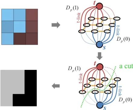
Figure 2.11 shows a simple example of 3×3 image for binary segmentation. First, we construct a graph based on the original image using unary term and smoothness term. Each pixel corresponds to a node in the graph. There are two special terminal nodes, the source node s and the sink node t, which represent the set of labels that can be assigned to each pixel. The thickness of the edges corresponds to the magnitude of the edge weights, i.e., thick edge represents large weight while thin edge represents small weight. There are two types of edges in the graph. One is between neighboring pixels, usually calledn−linkswhose weights reflect the penalty for discontinuity between neighboring pixels and are derived from the pair-wise smoothness term in the energy function. The other type of edges connect the pixel node and the terminal node, often called t −links whose weights represent the cost for being the corresponding label and are determined by the data term in the energy function.

Graph cuts can be used for optimizing the energy function that corresponds to the graph built previously. A minimum cut, labeling the pixels in the image into two disjoint sets, can be obtained. The two disjoint sets represent the binary segmentation, as shown in Figure 2.11.

Not all kinds of energy functions can be optimized by graph cuts, Kolmogorov [31] showed that only submodular energy functions can be optimized by graph cuts. In binary labeling case, the energy function needs to satisfy the following inequality:

Vpq(0,0)+Vpq(1,1)≤Vpq(1,0)+Vpq(0,1), (2.27)

where,{0,1}is the label set andVpqis the pair-wise smoothness term in the energy function

(46)

(47)

2.2.6 Volume Ballooning

In some cases, we may want to change the parameters of the energy function to obtain a large enough tumor segmentation, but changing the relative weight between the data term and the smoothness term may be insufficient to obtain larger segmentation results. This motivates us to incorporate volume ballooning into our approach to get larger tumor segmentation.

We adopt uniform ballooning [9] in our method. It is implemented by adding a bonus value in the data term for each pixel in the image if it is labeled as the foreground. For each pixel p, we add a term Bp(0) = βas an additional cost for being labeled as the background. Then, the

energy function, based on the approach adopted in [9], with volume ballooning becomes:

E(f)=X

p∈Ω

Dp(fp)+λ X

pq∈N

Vpq(fp, fq)+ X

p∈Ω

Bp(fp) (2.28)

Because Bp is the volumetric bias and an unary (linear) term, it is convenient to be included

(48)

Chapter 3 Automatic Brain Tumor Segmentation

Brain tumor segmentation is important in diagnosis and treatment of brain tumors. We inves-tigate automatic brain tumor segmentation by combining deep convolutional neural networks with regularization by a graph cut.

In this chapter, we present the details of our approach. First, we discuss how we apply several deep convolutional networks for brain tumor segmentation. Then, we describe how we apply graph cuts with different data terms to regularize the segmentation results obtained by neural networks.

3.1 Overview of our approach

First, we evaluate several different deep convolutional network architectures for the task of tumor segmentation. We train the networks on overlapping brain crops. We first tested on whole brain slices using the network trained on whole brain slices but it did not work well. Since the tumor pixels account for a very small portion in the whole brain slice, segmenting tumors from background is a highly imbalanced dense prediction task. We use the loss function that takes the imbalance of the training data into consideration by putting a higher weight for the loss incurred by the pixels whose true label is tumor. The next step is to combine the results on overlapping crops to obtain segmentation on a whole brain slice. We do this by a simple union operation.

Second, we apply graph cut regularization using the segmentation probability map obtained by deep convolutional neural networks to further improve the segmentation results obtained by deep neural networks. We explore and evaluate several ways in which the tumor probabilities learned by the neural networks can be converted to the data terms required by regularization a graph cut. We optimize all the parameters of the graph cuts segmentation by using grid search on the validation data.

(49)

36 Chapter3. AutomaticBrainTumorSegmentation

3.2 Deep CNNs for tumor segmentation

Since our labeled data is limited and a brain tumor is imbalanced in the whole slice, we crop the whole slices into overlapping small crops, as shown in Figure 3.1.

We experimented with different crop sizes and found through the experiments that training on crops of size 128× 128 is faster than larger crops and works comparably to training on larger crops. The crop size should consist of the factor that is the power of 2 because each pooling layer will decrease the resolution by half. The image crop is overlapped by half in one dimension with previous one. The experiment chapter shows how the crop size affects the accuracy of the segmentation. We make the crops overlap since any particular crop can contain only a part of a tumor, resulting in poor tumor detection. With overlap, a neighboring crop will have a larger or almost whole tumor, likely to give a better tumor detection. Then, we divide the whole dataset into training, validation and test sets. We choose and experiment with the deep convolutional neural network architectures that were previously successful for semantic segmentation and medical image segmentation, such as fully convolutional neural networks [36], deep dilated residual networks [58] and U-Net [46] on training data and validate its generalization performance on validation data. When making segmentation predictions on test data of whole brain slices, we still first predict the segmentation on overlapping crops that are exactly the same size and overlap as those used during training, i.e., by running forward propagation and getting the prediction score or probability map, then taking its maximum element index for each pixel as the segmentation prediction label. Then, we combine the segmentation results on the overlapping crops by a simple union operation.

3.2.1 Several Deep CNN Structures

(50)

3.2. DeepCNNs for tumor segmentation 37

Figure 3.1: Examples of overlapping crops. The boxes with different colors are the correspond-ing crops on the original image.

Fully Convolutional Network

A fully convolutional network (FCN) [39] is the network for which the learnable layers are only convolutional layers, and does not have any fully connected layers. There are several ad-vantages of FCN over convolutional networks with several fully connected layers. First, we can use various image sizes as input to the FCN, while convolutional networks with fully connected layers can only accept input images with a fixed size. Second, fully connected layers need lots of memory storage and numerical computation because lots of parameters need to be learned, while convolutional networks can learn good features and require much less parameters. Fully connected layers can be converted into convolutional layers by replacing fully connected layers with convolutional layers. Then, the whole network becomes fully convolutional.

While fully convolutional networks can be modified to perform semantic segmentation, their segmentation results are coarse. This issue is addressed by adding skips [6] that com-bine the final prediction layer with lower layers. This turns a line structure of convolutional neural network into a directed acyclic graph with edges that skip from lower layers to higher ones. Combining fine layers with coarse layers allows the model to fuse different levels of information, as suggested in [36].

Automatic Brain Tumor Segmentation by Deep Convolutional Networks and Graph Cuts

Scholarship@Western

Scholarship@Western

Automatic Brain Tumor Segmentation by Deep Convolutional

Automatic Brain Tumor Segmentation by Deep Convolutional

Networks and Graph Cuts

Networks and Graph Cuts

Abstract

Acknowledgement

Contents

List of Figures

List of Tables

List of Appendices

Chapter 1

Introduction

1.1

MRI and Brain Tumor

1.2

Challenge for Brain Tumor Segmentation

1.3

Overview of MRI-based Brain Tumor Segmentation

1.4

Convolutional Neural Network Approach for Brain

Tu-mor Segmentation

1.5

Our Approach

1.6

Outline of This Thesis

Chapter 2

Related Work

2.1

Deep Convolutional Neural Network

2.1.1

Convolution Operation

2.1.2

Dilated Convolution

2.1.3

Pooling

2.1.4

Batch Normalization

2.1.5

Training the neural networks

2.2

Energy Minimization Framework

2.2.1

Energy Minimization

2.2.2

Data Term

2.2.3

Smoothness Term

2.2.4

Optimization with Graph Cuts

2.2.5

Binary Segmentation with Graph Cut

2.2.6

Volume Ballooning

Chapter 3

Automatic Brain Tumor Segmentation

3.1

Overview of our approach

3.2

Deep CNNs for tumor segmentation

3.2.1

Several Deep CNN Structures