Parametric Co-variance Assignment for a Class of Multivariable Stochastic Uncertain Systems: Output Feedback Stabilization Approach

www.astesj.com

Special Issue on Multidisciplinary Sciences and Engineering

Parametric Co-variance Assignment for a Class of Multi-variable

Stochastic Uncertain Systems: Output Feedback Stabilization

Approach

Qichun Zhang*

School of Engineering and Sustainable Development, De Montfort University, Leicester, LE1 9BH, UK

A R T I C L E I N F O A B S T R A C T

Article history:

Received: 08 August, 2018 Accepted: 08 September, 2018 Online: 20 September, 2018 Keywords:

Reduced-order closed-form co-variance model

Parametric co-variance as-signment

Output feedback stabilization

This paper presents a novel parametric co-variance assignment strategy for multi-variable stochastic uncertain systems. Based upon the explicit parametric design and reduced-order closed-form co-variance model, the variances and co-variances of the system outputs can be assigned artifi-cially using output feedback while the effect of the system uncertainties can be minimized by optimizing the free parameters. In addition, the stability of the closed-loop system has been analyzed and an illustra-tive numerical example is given to demonstrate the effectiveness of the presented strategy. As a summary, the contributions of this paper in-clude the reduced-order co-variance model, the co-variance error based performance criterion and the parametric control design with stability analysis.

1

Introduction

Co-variance analysis permeates almost all of system theory [1]. Based on the co-variance analysis, the prob-abilistic properties among random signals can be de-scribed. Naturally, the associate co-variance control problem became one of the most significant research topics for multi-variable stochastic systems. Since the system identification, Kalman filtering, stochastic dis-tribution control and fault diagnosis are widely used in practice, the co-variance estimation and control are significant to all of these research areas and applica-tions [2, 3, 4, 5]. In addition, the co-variance is also an ideal tool to analyze the performance of the stochastic systems for the probabilistic decoupling analysis [6, 7] and neural interaction analysis [8, 9].

During the past two decades, the main result of co-variance control is based on the Lyapunov equation while several conditions and controllers have proposed the control design for the co-variance assignment using the determined control signals [10, 11]. However, this controller is designed by Lyapunov equation without closed-form formulation. Since the closed-form model of state co-variance [12] presented in 2007, reduced-order co-variance model [13] has been presented based on eigen-decomposition to solve output co-variance as-signment (OCA) problem while the co-variance model

was presented for the stochastic system with paramet-ric uncertainty. However, all the existing results did not consider the control design with parametric un-certainties of the stochastic systems. Considering the uncertainties of the parameters, the robust controller has been designed in [14, 15, 16]. All the mentioned controllers can achieve good performance, however these methods have not been used to deal with the co-variance analysis. To the best of our best knowledge, there is no existing solution to the parametric output-feedback co-variance assignment for stochastic uncer-tain systems with the stability analysis. Therefore, it is significant to develop a simply output co-variance as-signment (OCA) control law for the implementation of the complex dynamic multi-variable stochastic system with uncertainties.

In this paper, the stochastic uncertain multi-variable systems have been investigated while the co-variance assignment is very difficult since the uncer-tainties would affect the stability of the closed-loop systems. Based upon the investigated uncertain multi-variable model, the transformed co-variance model can be obtained firstly, and then the controller and linear observer can be designed and analyzed. In particular, the sufficient conditions are given for the convergence of the observer, the stabilization of the controller and

*_{Q. Zhang. Email:[email protected]}

stabilization of the closed-loop system, respectively. In the end, the control input can be obtained by re-versing the transformation. Using this control strategy, the design procedure is also given. Furthermore, the parameters of the controller and observer can be opti-mized using the parametric state feedback [17, 18] and entropy-based performance criterion. Using the pre-sented control strategy, the optimal output feedback control law is obtained for OCA and the performance has been verified by the numerical simulation.

The rest of the paper is organized as follows. In Section 2, the formulation is given including the model formulation, transformed co-variance model and con-trol objective. The parametric concon-trol strategy is de-veloped while the convergence of the linear observer, the stabilization of the parametric state feedback con-troller and the stabilization of closed-loop uncertain system are analyzed in Section 3. Moreover, the param-eter optimization and design procedure are also given in this section. Section 4 and Section 5 present the results of numerical simulation and the conclusions, respectively.

2

Formulation

Suppose that the complex industrial dynamic process can be modeled by the following stochastic uncertain multi-variable system.

dx(t) = (A+∆A(t))x(t)dt+ (B+∆B(t))u(t)dt+Ddβt

y(t) =Cx(t) (1)

wherex∈Rn,u∈Rsandy∈Rmare the system state

vector, input vector and output vector, respectively.βt

is thep-dimensional Wiener process. m,nandsare positive integers while system matricesA,B,C Dand parameter uncertainties∆A(t),∆B(t) are of appropri-ate dimensions.

Notice that the model (1) can be rewritten as fol-lows:

dx(t) = ((A+∆A(t))x(t) + (B+∆B(t))u(t) +Dw(t))dt y(t) =Cx(t) (2)

wherewis a standard Gaussian white noise. Without loss of generality, assume that the investigated system model (1) satisfies the following assumptions.

Assumption A1: Assume that the Gaussian noise vectorw(t) satisfies

E{_w(t)}_{= 0}

Enw(t)wT(t)o= 0

Enw(t)wT(τ)o=Qδ(t−_{τ) (3)}

whereδ(·_{) is the Dirac delta function.}

Assumption A2: Similar to the assumption of the noise, assume that the control signal is restricted by

E{_u(t)}_{= 0}

Enu(t)uT(t)o= 0

Enu(t)uT(τ)o=U(t)δ(t−_{τ) (4)}

whereU(t)=∆Enu(t)uT(t)o.

Based on the definition of the co-variance matrix, the state and output co-variance matrices of the given system are given by

Px(t) ∆

=Enx(t)xT(t)o

Py(t) ∆

=Eny(t)yT(t)o (5)

In addition, the co-variance matrices can be rewrit-ten as follows:

Px(t) =VxΛx(t)VxT

Py(t) =VyΛy(t)VyT

U(t) =VuΛu(t)VuT

Q=VqΛqVqT

(6)

whereΛ_x,Λ_y,Λ_u andΛ_qare real diagonal matrices.

Vx,Vy,Vu andVqare associated orthogonal matrices.

All of the matrices are with the same dimensions as the associated vectors.

Therefore, the reduced-order closed-form co-variance model can be obtained following the vector-ization operation.

˙

λx(t) = (Acov+∆Acov)λx(t) + (Bcov+∆Bcov)λu(t) +Dcovλq

λy(t) =Ccovλx(t)

(7) where λx, λy, λu and λq are the diagonal elements

of matricesΛ_x,Λ_y,Λ_u andΛ_q, respectively. The co-efficient matrices can be calculated using Hadamard product as follows:

Acov=AΛ ◦

AΛ

Bcov=BΛ ◦

BΛ

Dcov=DΛ ◦

DΛ

Ccov=CΛ ◦

CΛ

∆Acov=∆AΛ ◦

∆AΛ+ 2 (AΛ ◦

∆AΛ)

∆Bcov=∆BΛ ◦

∆BΛ+ 2 (BΛ ◦

∆AΛ)

(8)

while ∆AΛ = VxT∆AVx, ∆BΛ = VxT∆BVu, ∆CΛ =

VyT∆CVx,AΛ=VxTAVq,BΛ=VxTBVq,CΛ=VxTCVqand

DΛ=VxTDVq. Moreover, reserving the diagonal

ele-ments ofAΛwhich forms a diagonal matrixAdiag, then

Acov= 2Adiag. Similarly,∆Acov= 2∆Adiag.

Thus, the control objective is to develop a new con-trol strategy to assign the state of the transformed model (7) so that the covariances and variances of the system outputs can be assigned simultaneously.

To achieve the mentioned control objective, the fol-lowing assumption should be taken into account:

Assumption A3: The pair (Acov, Bcov) is control-lable.

Assumption A4: The admissible parameter uncer-tainties are of the norm-bounded form

h

∆Acov(t) ∆Bcov(t) i

=Mh Ξ₁(t)N1 Ξ2(t)N2 i

(9)

with proper dimensions.Ξ₁(t) andΞ₂(t) are unknown time-varying matrices which respectively meet the fol-lowing conditions.

ΞT₁(t)Ξ₁(t)≤_I,ΞT

2(t)Ξ2(t)≤I (10)

In addition, the following lemma [19] has been recalled here which can be used to analyze the con-vergence and stabilization of the presented control strategy.

Lemma 1. Given any real constant matricesX andY with proper dimensions. Then there exists a constant ξ >0, such that the following inequality holds.

XTY+YTX≤_ξXT_X+ξ−1_YT_{Y (11)}

3

Control Strategy

The reference co-variance matrix can be rewritten as follows:

R=VrΛrVrT (12)

Since the diagonal matrix r can be arranged as vector

λr, the co-variance assignment problem transfers to

state tracking problem using the presented reduced-order co-variance model if we setVy=Vr.

To track the desired state co-variance vector, the integrator should be considered in the control scheme. The error vectorey(t) =λrλyis treated as the extended

state and substitutes the error into the closed-loop sys-tem.

Then, the closed-loop system in the state-space form can be obtained as follows:

" _˙

λx(t)

˙¯

ey(t)

#

=A¯+∆A¯

"

λx(t)

¯

ey(t)

#

+B¯+∆B¯λu(t)

+ ¯Dλq+

" 0

λr

#

λy(t) = ¯C

"

λx(t)

¯

ey(t)

#

(13)

where

¯

A= "

Acov 0

−_{Ccov 0}

#

,B¯= "

Bcov 0

#

,C¯ = "

CcovT 0

#T

¯

D= "

Dcov 0

#

∆A¯= "

∆Acov 0

0 0

#

,∆B¯= "

∆Bcov 0

#

(14)

and

˙¯

ey(t) =ey(t) (15)

We can further present the closed-loop system in compact format as follows:

˙¯

x(t) =A¯+∆A¯x¯(t) +B¯+∆B¯λu(t) + ¯Dλq+ ¯λr

λy(t) = ¯Cx¯(t) (16)

where

¯

x(t) = "

λx(t)

¯

ey(t)

#

,λ¯r=

" 0

λr

#

(17)

Notice that ¯Dλq and ¯λr are real constants which

means that if the following system is stabilized then the variance and co-variance assignment can be com-pleted.

˙¯

x(t) =A¯+∆A¯x¯(t) +B¯+∆B¯λu(t)

λy(t) = ¯Cx¯(t) (18)

Based upon the transformed system model 18, the control strategy can be divided into two parts: observer-based output feedback design and the parametric opti-mization for uncertainty compensation.

3.1

State feedback design

The linear state feedback controller can be determined by the nominal linear model and the control law is described by

λu(t) =Kx¯(t) (19)

where the gain matrixKcan be obtained by parametric design [17, 13]. In particular, we have

K= [W1f1, . . . , Wmfm]

×h_(λ∗

1I−A1)

−₁

B1f1, . . . ,(λ

∗

mI−Am) −₁

Bmfm

i−1 (20)

where modified parameter vectors and closed-loop eigenvalues are denoted by f1, . . . , fm and λ

∗

1, . . . , λ

∗ m

which can be considered as free parameters. In the case of a common open-loop and closed-loop eigen-value, the gain matrixK can be determined by the following equations.

Aj= ¯A+vj0w0j T

Wj=I−

eiw0j T _¯

B

w0_jTbi

Bj= ¯BWj+v0jeTi , j= 1, . . . , m (21)

where v_j0 andw0_j denote the open-loop eigenvectors and eigenrows ofAj. bi is thei-th column of ¯B. ei is

a unit vector while thei-th element is 1. In the other case, no common eigenvalue results inw0_jTbi= 0 which

leads to

Aj= ¯A

Wj=I

Bj= ¯B, j= 1, . . . , m (22)

Substituting control law (19) into the transformed system model (18) yields the closed-loop system:

˙¯

x(t) = (Ac+∆Ac(t))x(t) (23)

whereAc= ¯A+ ¯BK,∆Ac(t) =∆A¯(t) +∆B¯(t)K. Thus the

Lemma 2. For the uncertain multi-variable system given by (18), with the assumptions and with the control law given by (19), then there exist two positive constantsε1

andε2, so that the equilibriumx¯(t) = 0is stabilized if the

following matrix inequality has a positive-definite solution P =PT >0.

ATcP +P Ac+ε1N1TN1+

ε−₁1+ε₂−1P MMTP

+ε2KTN2TN2K+ε3PTP <0 (24)

Proof. Consider the Lyapunov function candidate as

Vc( ¯x) = ¯xT(t)Px¯(t), P =PT >0 (25)

The time derivative ofVc( ¯x) along the trajectories

of (23) is given as follows. ˙

Vc( ¯x) = ¯xT(t)ATcPx¯(t) + ¯xT(t)P Acx¯(t)

+ ¯xT(t)∆A¯T(t)Px¯(t) +xT(t)P∆A¯(t) ¯x(t)

+ ¯xT(t)KT∆B¯T(t)Px¯(t) + ¯xT(t)P∆B¯(t)Kx¯(t) (26)

Letε1andε2be positive constants, the following matrix inequalities hold using Lemma 1.

¯

xT(t)∆A¯T(t)Px¯(t) +xT(t)P∆A¯(t) ¯x(t)

= ¯xT(t) (MΞ1N1)TPx¯(t) + ¯xT(t)pMΞ1N1x¯(t)

≤_x¯T_{(t) (ε1N}T

1N1+ε

−1

1 P MMTP) ¯x(t) (27)

¯

xT(t)KT∆B¯T(t)Px¯(t) + ¯xT(t)P∆B¯(t)Kx¯(t)

= ¯xT(t)KT(MΞ₂N2)TPx¯(t) + ¯xT(t)P MΞ2N2Kx¯(t)

≤_x¯T_{(t) (ε2K}T_N2T_N2K+ε−₂1_{P MM}T_{P) ¯x(t) (28)}

Substituting these inequalities into the derivative ofVc( ¯x) with Assumption 4, we have

˙

Vc( ¯x)≤x¯T(t)

AT_cP +P Ac

¯

x(t)

+ ¯xT(t)ε1N1TN1+ε

−₁

1 P MMTP

¯

x(t)

+ ¯xT(t)ε2KTN2TN2K+ε

−₁

2 P MMTP

¯

x(t) (29)

Since ˙Vc( ¯x) < 0 , the proof of lemma 2 is

com-pleted.

3.2

Observer design

Using the linear observer to estimate the states of the model (18), the linear observer can be designed based on the nominal linear model.

˙ˆ¯

x(t) =A¯−_LC¯_{xˆ¯(t) +Lλy(t) + ¯Bλu(t) (30)}

where the estimated vector can be denoted by ˆ¯xandL

is pre-specified gain matrix of this observer. Introducing the error of the estimation by

e(t) = ¯x(t)−_{xˆ¯(t) (31)}

and substituting the Eq. (30)-(31) to system model (18). The closed-loop model can be described by

˙

e(t) =Aoe(t) +∆Ac(t) ¯x(t) (32)

whereAo= ¯A−LC¯. Similar to Lemma 2, Lemma 3 is

given as follows.

Lemma 3. For the uncertain multi-variable system given by (18), with the assumptions and with the linear observer given by (30), then there exists two positive constantsε1

andε2, so that the estimation errore(t)converges to zero

if the following matrix inequalities have a positive-definite solutionP =PT >0.

AoP+P Ao<0

(33)

ε1N1TN1+

ε₁−1+ε−₂1P MMTP+ε2KTN2TN2K <0 (34)

Proof. Consider the Lyapunov function candidate as

Vo(e) =eT(t)P e(t), P =PT >0 (35)

The time derivative ofVo(e) along the trajectories

of (31) is given by the following equation.

˙

Vo(e) =eT(t) (AoP+P Ao)e(t)

+ ¯xT(t)∆A¯T(t)Px¯(t) + ¯xT(t)P∆A¯(t) ¯x(t)

+ ¯xT(t)KT∆B¯T(t)Px¯(t) + ¯xT(t)P∆B¯(t)Kx¯(t) (36)

Similar to the proof of Lemma 2, we have

˙

Vo(e)≤eT(t) (AoP+P Ao)e(t)

+ ¯xT(t)ε1N1TN1+ε

−₁

1 P MMTP

¯

x(t)

+ ¯xT(t)ε2KTN2TN2K+ε

−₁

2 P MMTP

¯

x(t) (37)

which ends the proof

3.3

Output feedback design

Combining the parametric state feedback controller and the designed observer, the output feedback con-troller can be obtained for the system (18).

λu(t) =Kxˆ¯(t) (38)

which leads to the closed-loop dynamics as follows.

˙¯

x(t) =Acx¯(t) +∆Ac(t) ¯x(t)−

¯

B+∆B¯(t)Ke(t) (39)

Furthermore, the stability of the closed-loop con-trol design can be guaranteed by the following theo-rem.

Theorem 4. For the uncertain multi-variable system given by (18), with the assumptions and with the con-trol law given by (38) using the observer (30), then there exists two sets of positive constants εi, i = 1, . . . ,2 and

εj, j= 4, . . . ,7, so that the equilibriumx¯(t) = 0is stabilized

if the following matrix inequalities have positive-definite solutionP1=P1T >0, P2=P2T >0.

ε4KTBTBK+ε5KTN2TN2K+AoP2+P2Ao+ε8P2TP2<0 (40)

ATcP1+P1Ac+ (ε −1 1 +ε

−1 2 +ε

−1 4 +ε

−1

5 )P1MMTP +ε−₆1+ε₇−1P2MMTP2+ (ε2+ε7)KTN2TN2K

+ε3P1TP1+ (ε

−1 3 +ε

−1

Proof. Consider the Lyapunov function candidate as

V( ¯x(t), e(t)) = ¯xT(t)P1x¯(t) +eT(t)P2e(t) (42)

The time derivative ofV( ¯x(t), e(t)) along the trajecto-ries of (39) is shown as follows.

˙

V( ¯x(t), e(t)) = ¯xTATcPx¯+ ¯xTP Acx¯

+ ¯xT∆A¯TPx¯+ ¯xTP∆A¯x¯

+ ¯xTKT∆B¯TPx¯+ ¯xTP∆BK¯ x¯−_eT_KT_B¯T_Px¯ −_x¯T_PBKe¯ −_eT_KT_∆B¯T_Px¯−_x¯T_P∆BKe¯

+eT(t) (AoP +P Ao)e(t)

+ ¯xT(t)∆A¯T(t)Px¯(t)

+ ¯xT(t)P∆A¯(t) ¯x(t) + ¯xT(t)KT∆B¯T(t)Px¯(t) + ¯xT(t)P∆B¯(t)Kx¯(t) (43)

Letε4andε5be positive constants, the following ma-trix inequalities hold using Lemma 1.

−_eT_(t)KT_B¯T_Px¯(t)−_x¯T_(t)PBKe¯ _(t)

≤_ε4eT_(t)KT_B¯T_BKe¯ _{(t) +ε}−1

4 x¯T(t)P MMTPx¯(t) (44)

−_eT_(t)KT_∆B¯T_(t)Px¯(t)−_x¯T_(t)P∆B¯_(t)Ke(t) ≤_ε5eT_(t)KT_NT

2N2Ke(t) +ε

−₁

5 x¯T(t)P MMTPx¯(t) (45)

Substituting these inequalities into the derivative ofV( ¯x(t), e(t)) and using Lemma 3, we have

˙

V ≤_x¯T_{(t) [A}T_{cP1+P1Ac+ (ε1+ε6)N}T

1N1 + (ε2+ε7)KTN2TN2K

+ (ε−11+ε

−₁

2 +ε

−₁

4 +ε

−₁

5 )P1MMTP1 +ε−₆1+ε₇−1P2MMTP2] ¯x(t)

+eT(t) (ε4KTB¯TBK¯ +ε5KTN2TN2K

+AoP2+P2Ao)e(t) (46)

which leads to the conditions and the proof has been

completed.

3.4

Parametric optimization

Notice that all the free parameters can be adjusted without changing the stability of the system, which means that the optimization of the parameters can be done for various performance criteria. In this paper, we design the controller based on the nominal model then the optimization can be considered as the uncer-tainty compensation using the following performance criterion.

J= Z t

0

R1E n

ey(t)

o +R2H

n

ey(t)

o

dt (47)

where real positiveR1 andR2 stand for the weights.

H{·}_{denotes the entropy. To simplify the performance}

criterion, the entropy can further be replaced equiva-lently by information potential [20, 21].

Then the optimal free parameterfi can be obtained

by gradient descent once the eigenvaluesλ∗_i are pre-specified.

fi,j+1=fi,j+µ

dJ dfi

_f

i=fi,j

i= 1, . . . , m (48)

wherejdenotes the optimization searching iteration index.µstands for the pre-specified step.

Once the control law λu is obtained, the control

inputu(t) for system (1) can be calculated by reversing the transformation. In particular,Λ_U can be obtained byλu and we have

u(t) =hVuΛˆu(t)VuT

i1₂

ξ(t) (49)

whereξ(t) denotes the standard Gaussian white noise.

Remark 1. The actual control law is non-linear though the transformed system model is linear.

Remark 2. Based on the dual principle, the observer gain matrix can be also obtained using proposed optimization approach. Meanwhile, the optimization operation can also be replaced by multi-objective optimization algorithms then the weights can be neglected.

Remark 3. Only a few elements of the parameter vectors fi affect the control performance directly. Therefore, in

order to determine the free parameters quickly, trial and error method can be used and the performance criterion can verify the manually selected parameters simply.

3.5

Design procedure

The procedure of the proposed control strategy is sum-marized as follows:

Step1 Transfer the system to co-variance assignment model.

Step2 Setup the initial free parameters of the controller.

Step3 Use the numerical approach to optimize the per-formance criterion (47), by computing the mean, the entropy and gradient descent, then the opti-mal parameters are obtained.

Step4 Update the feedback gain matrix of the control law (19, 49), and verify it by the conditions of Lemma 2 to guarantee stability of the system, if the conditions hold, then go to next step, other-wise, return to Step 1.

Step5 Obtain the feedback gain matrix of the observer by dual principle and verify it by Lemma 3.

Step6 Verify the optimal parameters by Theorem 4, and if the conditions can be satisfied, then complete the procedure, otherwise, return to Step 2.

4

A Numerical Simulation

To verify this new model and the control algorithms proposed in this paper, one numerical example is pre-sented in this section.

The original model can be shown as below:

A= "

−_0.5 −_0.3

0.1 −_0.2

#

, B= "

2 0.3 0.1 4

#

C= "

0.7 0.1 0.2 0.8

#

, D= "

0.1 0 0 0.1

#

The co-variance matrix of disturbance white noises

is _"

0.2 0.1 0.1 0.2

#

To assign the co-variance matrix, we choose the reference co-variance matrix as

"

0.2 0.1 0.1 0.3

#

The parametric uncertainties are given as follows:

Ξ₁(t) =Ξ₂(t) =Isint

N1= "

0.1 0 0 0.1

#

, N2= "

0.2 0 0 0.1

#

Simply, we have

λr=

"

0.1382 0.3618

#

We can further obtain the eigen-vector of the variables as follows:

Vr=Vy=Vx=Vu=Vq=

"

−_{0.8507 0.5257}

0.5257 0.8507 #

0 5 10 15 20 25 30 35 40

Time (s)

-0.05 0 0.05 0.1 0.15 0.2 0.25 0.3 0.35 0.4

x₁ Variance

x₁/x₂ Co-variance x

2 Variance

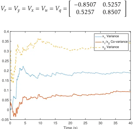
Figure 1. The measured co-variance and variances of the system outputs.

Following the presented control strategy, the sim-ulation results have been shown by Fig. 1-4. Partic-ularly, Fig. 1 indicates the co-variance and variances of the system outputs. Comparing to the reference co-variance matrix, the practical system outputs achieve the assignment with uncertainties. Meanwhile, Fig.

2 shows that the system outputs are stable if the transformed co-variance system design is stabilized while the states and control inputs of the transformed co-variance model have been given by Fig. 3 and Fig. 4. It has been shown that the eigenvalues of the co-variance matrix are tracking the reference eigen-values of the reference co-variance matrix and the practical control input can be obtained by reversing the transformation using the values of the designed control input of the transformed co-variance model.

0 5 10 15 20 25 30 35 40

Time (s)

-2 -1.5 -1 -0.5 0 0.5 1 1.5 2 2.5

y

1

y

2

Figure 2. The outputs of the system.

0 5 10 15 20 25 30 35 40

Time (s) 0

0.05 0.1 0.15 0.2 0.25 0.3 0.35 0.4

x 1 x 2

Figure 3. The state assignment of the transformed co-variance model.

0 5 10 15 20 25 30 35 40

Time (s) 0

0.005 0.01 0.015 0.02 0.025

u1

u2

5

Conclusion

This paper investigates the co-variance assignment strategy for a class of multi-variable stochastic un-certain systems. Combining the reduced-order co-variance model and parametric feedback, the control strategy is obtained by output feedback stabilization. In particular, the transformed model is given firstly with the extended co-variance assignment error. Then the linear observer is designed to estimated the ex-tended state of the transformed model. After that, the output feedback is obtained via parametric opti-mization. Meanwhile the theoretical analysis is given to guarantee the robustness, stabilization and conver-gence of the closed-loop systems. Based on the results of the numerical simulation, the effectiveness of the presented control strategy has been verified while the control objectives have been achieved. Since the co-variance assignment is widely used in practical sys-tems, such as paper-making process, the industrial applications using the presented control strategy will be the potential extension as a future work.

Conflict of Interest The authors declare no conflict of interest.

Acknowledgement The authors would like to thank the anonymous reviewers for their valuable com-ments.

References

[1] A. Hotz and R. E. Skelton, “Covariance control theory,” Inter-national Journal of Control, vol. 46, no. 1, pp. 13–32, 1987.

[2] K. Liu, K. Li, and C. Zhang, “Constrained generalized predic-tive control of battery charging process based on a coupled thermoelectric model,”Journal of Power Sources, vol. 347, pp. 145–158, 2017.

[3] M. Ren, J. Zhang, M. Jiang, M. Yu, and J. Xu, “Minimum (hphi)– entropy control for non-gaussian stochastic networked control systems and its application to a networked dc motor control sys-tem,”IEEE Transactions on Control Systems Technology, vol. 23, no. 1, pp. 406–411, 2015.

[4] L. Guo, L. Yin, H. Wang, and T. Chai, “Entropy optimization filtering for fault isolation of nonlinear non-gaussian stochastic systems,”IEEE Transactions on Automatic Control, vol. 54, no. 4, pp. 804–810, 2009.

[5] L. Yao, J. Qin, H. Wang, and B. Jiang, “Design of new fault diagnosis and fault tolerant control scheme for non-gaussian singular stochastic distribution systems,”Automatica, vol. 48, no. 9, pp. 2305–2313, 2012.

[6] Q. Zhang, J. Zhou, H. Wang, and T. Chai, “Minimized coupling in probability sense for a class of multivariate dynamic stochas-tic control systems,” inDecision and Control (CDC), 2015 IEEE 54th Annual Conference on. IEEE, 2015, pp. 1846–1851. [7] ——, “Output feedback stabilization for a class of

multi-variable bilinear stochastic systems with stochastic coupling attenuation,”IEEE Transactions on Automatic Control, vol. 62, no. 6, pp. 2936–2942, 2017.

[8] Q. Zhang and F. Sepulveda, “A statistical description of pair-wise interaction between nerve fibres?” inNeural Engineering (NER), 2017 8th International IEEE/EMBS Conference on. IEEE, 2017, pp. 194–198.

[9] ——, “A model study of the neural interaction via mutual coupling factor identification,” inEngineering in Medicine and Biology Society (EMBC), 2017 39th Annual International Confer-ence of the IEEE. IEEE, 2017, pp. 3329–3332.

[10] K. Yasuda and R. E. Skelton, “Covariance controllers: A new parameterization of the class of all stabilizing controllers,” in

American Control Conference, 1990. IEEE, 1990, pp. 824–829. [11] K. M. Grigoriadis and R. E. Skelton, “Minimum-energy co-variance controllers,”Automatica, vol. 33, no. 4, pp. 569–578, 1997.

[12] H. Khaloozadeh and S. Baromand, “State covariance assign-ment problem,”IET control theory & applications, vol. 4, no. 3, pp. 391–402, 2010.

[13] Q. Zhang, Z. Wang, and H. Wang, “Parametric covariance assignment using a reduced-order closed-form covariance model,”Systems Science & Control Engineering, vol. 4, no. 1, pp. 78–86, 2016.

[14] Z. Wang, B. Huang, and H. Unbehauen, “Robust reliable con-trol for a class of uncertain nonlinear state-delayed systems,”

Automatica, vol. 35, no. 5, pp. 955–963, 1999.

[15] T. Shen and K. Tamura, “Robust h/sub/spl infin//control of un-certain nonlinear system via state feedback,”IEEE Transactions on Automatic Control, vol. 40, no. 4, pp. 766–768, 1995.

[16] Q. Zhang and X. Yin, “Observer-based parametric decoupling controller design for a class of multi-variable non-linear un-certain systems,”Systems Science & Control Engineering, vol. 6, no. 1, pp. 258–267, 2018.

[17] G. Roppenecker, “On parametric state feedback design,” Inter-national Journal of Control, vol. 43, no. 3, pp. 793–804, 1986. [18] G. Roppenecker and J. O’reilly, “Parametric output feedback

controller design,”Automatica, vol. 25, no. 2, pp. 259–265, 1989.

[19] I. R. Petersen, “A stabilization algorithm for a class of uncer-tain linear systems,”Systems & Control Letters, vol. 8, no. 4, pp. 351–357, 1987.

[20] Q. Zhang and A. Wang, “Decoupling control in statistical sense: minimised mutual information algorithm,”International Jour-nal of Advanced Mechatronic Systems, vol. 7, no. 2, pp. 61–70, 2016.