ULTRA-WEAK VARIATIONAL FORMULATION AND EFFICIENT INTEGRAL
REPRESENTATION IN ELECTROMAGNETISM: A THOROUGH STUDY OF
THE ALGORITHM COMPLEXITY
E. Darrigrand
1Abstract. Many different methods have been developed for the solution of the time-harmonic Maxwell equations in exterior domains at high frequency. Volume based methods have the drawback of needing an artificial boundary far from the obstacle. Integral formulations enable one to avoid this difficulty by solving a problem on the surface of the obstacle, but imply dense systems with bad condition numbers. In this paper we study a coupling of the Ultra-Weak Variational Formulation (UWVF), a volume based method using plane wave basis functions, and an integral representation of the unknown field to obtain an exact artificial boundary condition. More precisely, we detail the study of the complexity of the new algorithm considering a 1-level or multilevel Fast Multipole Method.
R´esum´e. La r´esolution des ´equations de Maxwell en r´egime harmonique en domaine ext´erieur, `a haute fr´equence, a induit de nombreuses m´ethodes dont les m´ethodes volumiques n´ecessitant la consid´eration d’une fronti`ere artificielle pour d´elimiter le domaine ext´erieur, ainsi que les formulations int´egrales ´evitant la consid´eration du domaine ext´erieur mais impliquant des syst`emes pleins g´en´eralement mal
conditionn´es. Dans cet article, nous ´etudions en d´etail les gains algorithmiques apport´es par le
couplage d’une m´ethode de r´esolution volumique, la formulation variationnelle ultra-faible, et d’une repr´esentation int´egrale, via l’utilisation de m´ethodes multipˆoles rapides.
Introduction
The Ultra-Weak Variational Formulation (UWVF) is a volume based numerical method for solving the time-harmonic Maxwell system on a bounded domain developed by B. Despr´es and O. Cessenat ( [2,3]). It uses local plane wave solutions on a finite element mesh to approximate the field. By varying the number of plane wave basis functions from element to element the UWVF can discretize the electromagnetic field with a coarser volume mesh in comparison to more classical methods like low order finite elements or finite differences. However, to approximate scattering on an unbounded domain, the UWVF requires an artificial boundary Γext sufficiently far from the obstacle. A simple absorbing boundary condition on Γext (as used in the original UWVF) implies a large domain around the obstacle and so a large number of degrees of freedom.
As we suggested in [7], in this paper we consider the use of an integral representation of the unknown field on Γext due to the method of C. Hazard and M. Lenoir ( [9]) extended by J. Liu and L. Jin ( [10]). In particular, their idea is to use an integral representation of the unknown on the artificial boundary Γext thanks to the unknown field values on a third boundary Σ taken closer to the boundary Γint. This couples the degrees of freedom on Σ to those on Γext. The main constraint is that the domain between Σ and Γextbe homogeneous (i.e. the background medium). Note that if the exterior domain is entirely homogeneous and we use the perfectly
1 IRMAR - Universit´e de Rennes 1, Campus de Beaulieu, 35042 Rennes cedex, France
c
EDP Sciences, SMAI 2007
Ω Γint
Γ ext
Σ
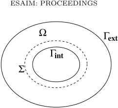
Figure 1. The exterior domain Ω
conducting boundary condition on Γint, we may take Σ = Γint. The artificial boundary Γext can then be taken very close to the boundary of the obstacle. However, this method requires the evaluation of integral operators which are expensive by direct means. We shall show that the use of the integral representation does not greatly increase the cost of the UWVF if the integral calculation is performed using a Fast Multipole Method (FMM) (see for example [4], [11], [8]). Indeed, for a given accuracy, the numerical complexity of the new algorithm is better than the complexity of the standard UWVF with a simple absorbing boundary condition on Γext. The first section gives a brief presentation of the UWVF. In Section 2, we describe the use of the integral representation within the UWVF, and give a thorough study of the complexity of the new algorithm using a 1-level or multilevel FMM, using or not a double-mesh concept, avoiding or not close interactions in the FMM. The last section presents encouraging numerical results obtained using a 1-level FMM in agreement with the study of the complexity.
1.
Ultra-Weak Variational Formulation
To solve a scattering problem for the time-harmonic Maxwell equations in a domain Ω we need to find the electric fieldE and magnetic fieldH such that the following equations hold: (see Fig. 1)
∇ ∧E−ıωµH =−m , ∇ ∧H+ıωεE=j , ∇ ·(εE) = 0, ∇ ·(µH) = 0,
in Ω, (1)
where m and j are given data functions specifying the current sources, ε and µ are positive functions of position and ω >0 is the angular frequency of the field. For use with the UWVF, the boundary condition on
∂Ω = Γint∪Γext is written in the following non standard form ( [3])
− |√ε|E∧ν+ (|√µ|H∧ν)∧ν =Q(|√ε|E∧ν+ (|√µ|H∧ν)∧ν) +g , (2)
where Q = 0 on Γext and g is computed from the incident wave to give a low order Absorbing Boundary Condition (ABC). Since we wish to model the total field we chooseg= 0 on Γint and useQto set the boundary condition. For example choosingQ= 1 gives the perfectly conducting boundary condition, while|Q|<1 gives an impedance condition.
The UWVF is based on the decomposition of the domain Ω into tetrahedra {Ωk}k=1,...,K and its unknown
is defined on the boundaries of these tetrahedra. This variational formulation is defined on the Hilbert space
V = QKk=1L2
t(∂Ωk) where L2t(∂Ωk) is the space of square integrable tangential fields on ∂Ωk the boundary
of Ωk, and the scalar product is given by (X,Y)V =PkR∂ΩkX/∂ΩkY/∂Ωk. Under the assumption thatε and
µ are positive constants on each Ωk, (E, H) is found through the restriction of the field (Ek, Hk) to ∂Ωk,
where (Ek, Hk) = (E, H)/Ωk. The method then solves for an unknown impedance trace X ∈ V, defined by
X/∂Ωk ∈L 2
t(∂Ωk) and
X/∂Ωk=
√ε
/∂Ωk(Ek∧νk) +
õ
whereε/∂Ωk andµ/∂Ωk are quantities defined by the values ofεandµon each side of∂Ωk (see [7] for details),
andνk is the exterior normal to∂Ωk.
The UWVF of Maxwell’s equations ( [2, 3]) is then to findX ∈V such that
(X,Y)V −(ΠX, FY)V = (eb,Y)V for allY ∈V, (4)
for allY ∈V given byY/∂Ωk =
√ε
/∂Ωk(E
′
k∧νk) +√µ/∂Ωk((H
′
k∧νk)∧νk) where the fields (Ek′, H ′
k) satisfy the
adjoint Maxwell problem
∇ ∧E′
k−ıωµΩkH
′
k = 0 in Ωk,
∇ ∧H′
k+ıωεΩkE
′
k = 0 in Ωk,
In (4),eb∈V is derived from the right hand side of (1) andggiven in (2). Π and F are local operators defined in [7] following [2, 3], such that Π is the one which involves the boundary condition (2) through the functionQ. By taking a finite dimensional subspaceVh⊂V and using basis functionsZi, i∈J, a Galerkin discretization
of the formulation (4) leads to problem of findingXh=Pi∈JXiZi∈Vhsuch that (Xh,Yh)V −(ΠXh, FYh)V =
(eb,Yh)V for allYh∈Vh.Equivalently, in matrix/vector form we seek to computeX = [X1,· · · , Xcard(J)]T such that
(D−C)X=b , (5)
where D is the matrix with (i, j)th entry (Zj, Zi)V andC has (i, j)th entry given by (ΠZj, F Zi)V. The data
vectorb is derived from the right hand side above in the same way.
As usual for the UWVF, on each Ωk we use a basis generated by taking the impedance trace of pk plane
waves satisfying the adjoint Maxwell system on Ωk (pk/2 directions with two polarizations for each direction).
At least six plane waves (and usually more) are used per element.
The UWVF then leads to a system of size (PKk=1pk). The number of plane waves pk must be chosen
depending on the local wavelength and diameter of the element. Suppose the electromagnetic parameters of the domain are constant and define the wave number κ=ω√εµ. The UWVF enables one to reduce the number of elements in the mesh, in comparison with a more classical volume method. Of course, the complexity of the method is then linked to the number of elements in the mesh and the number of basis functions per element. Let us introduce another parameter: K0 denotes the average number of tetrahedra taken in one dimension so that K ∼K3
0. As a volume method, the UWVF method leads to a sparse system. The number of degrees of freedom is of orderK3
0pand the complexity of the algorithm isO(K03p2) wherepdenotes the average number of basis functions per tetrahedra which typically satisfiesK0p∼κ.
2.
Use of an Integral Representation within the UWVF
For simplicity, we now suppose ε = µ = 1 so that Σ can be taken equal to Γint (i.e. the scatterer is not penetrable and the exterior medium is homogeneous). The idea presented by C. Hazard and M. Lenoir in [9] consists in replacing the low order absorbing boundary condition−E∧ν+ (H∧ν)∧ν =−E0∧ν+ (H0∧ν)∧ν on Γext by the boundary condition
−E∧ν+ (H ∧ν)∧ν=−Es∧ν+(Hs∧ν)∧ν−E0∧ν+(H0∧ν)∧ν ,
where (Es, Hs) are given by the Stratton-Chu formula ( [5]) in terms of field values on Σ = Γ
int via
Es(x) =∇
x∧
Z
Γint
G(x, y)νΣ(y)∧E(y)dγ(y)−
1
ı ω∇x∧ ∇x∧
Z
Γint
G(x, y)νΣ(y)∧H(y)dγ(y), (6)
Hs(x) =∇x∧
Z
Γint
G(x, y)νΣ(y)∧H(y)dγ(y) +
1
ı ω∇x∧ ∇x∧
Z
Γint
where νΣ is the exterior normal to the surface Σ = Γint and G(x, y) = exp(ıκ|x−y|)/(4π|x−y|) is the fundamental solution for the Helmholtz equation. Thanks to the structure of the unknown of the UWVF, as shown in [7], the fields in the integrands above can be computed directly from the degrees of freedom of the UWVF (3) taking into account the convention for the direction of normals, and the boundary condition on Γint (2) whereg= 0.
The system (5) becomes (D−C−Ce)X =b whereCe couples the degrees of freedom on Γint and Γext. The matrixCe can be split into different discrete integral operatorsCei, i= 1, ...,4 of the form
(CeiXh)kl =
Z
Σextkk
ckSi(Xh) · FYkldγext,
where
· Σextkk is the face on Γext of a tetrahedron which interacts with the exterior boundary,
· ck depends only onεandµon Σextkk,
· F is the local operator introduced in (4),
· Si is a global opertator which comes from the right hand side of (6)-(7), for instance
(S1(X))(x) = − Z
Γint
fQ(y)∇yG(x, y)∧ X(y)dγ(y)
!
∧ν(x),
wherefQ is a function involvingQandε. These integral operators can be evaluated by the FMM.
In this paper, the solution of the new system (D−C−Ce)X=bis obtained by the same method (BiCGStab) as used for the classical UWVF system (D−C)X =b, consideringC+Ce as a small perturbation ofC.
The integral representation aims to reduce the distance of the absorbing boundary from the scatterer to a number of elements independent of κ. We then have a number of elements in the mesh of order K2
0. This reduces the complexity related to the volume calculation. However the cost of the integral calculation would be very large unless treated carefully since the integral operators give rise to a matrix with large dense blocks. This cost is controlled thanks to the FMM.
A thorough study of the complexity of the new algorithm
In this paper, we focus on the complexity of the different methods. The number of basis functions per tetrahedron is supposed to be chosen depending on the wavenumber κ and the diameter of the concerned tetrahedron. The UWVF enables one to use a relative coarse mesh compared to more classical methods but the coarseness of the mesh is compensated by the choice of the number of basis functions per tetrahedron. Typically, in a global point of vue, the relationK0∼κof a classical method becomesK0p∼κfor the UWVF. As we mentioned in Section 1, the complexity of the UWVF method then writes O(K3
0p2) which corresponds toO(K0κ2).
The reduction of the thickness of the domain due to the integral representation leads to a number of tetra-hedra of orderK2
0. The resulting complexity of the volume calculation is then O(K02p2) which corresponds to
O(κ2). However, the calculation related to the integral representation leads to the complexityO(K4
0p2). Indeed, the number of tetrahedra connected to Γint or Γext is of orderK02. The FMM was introduced to accelerate such calculation. Using a 1-level FMM ( [4]) (resp. a multilevel FMM ( [8, 11])), the cost is reduced toO(K3
0p) (resp. O(K2
0ln 2
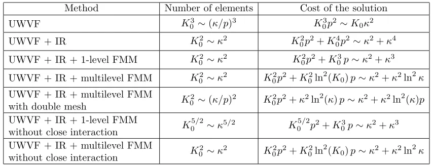
Complexity estimates for the methods in this paper
Method Number of elements Cost of the solution
UWVF K3
0 ∼(κ/p)3 K03p2∼K0κ2
UWVF + IR K2
0 ∼κ2 K02p2+K04p2∼κ2+κ4
UWVF + IR + 1-level FMM K2
0 ∼κ2 K02p2+K03p∼κ2+κ3
UWVF + IR + multilevel FMM K2
0 ∼κ2 K02p2+K02ln2(K0)p∼κ2+κ2ln2κ
UWVF + IR + multilevel FMM
with double mesh K 2
0 ∼(κ/p)2 K02p2+κ2ln 2
(κ)p∼κ2+κ2ln2 (κ)p
UWVF + IR + 1-level FMM
without close interaction K 5/2
0 ∼κ5/2 K
5/2
0 p2+K03p∼κ2+κ3
UWVF + IR + multilevel FMM
without close interaction K 2
0 ∼κ2 K02p2+K02ln 2
(K0)p∼κ2+κ2ln2κ
complexity O(κ3) with a 1-level FMM and O(κ2lnκ) with a multilevel FMM. The lost of the UWVF ability to consider a coarse mesh may be avoided by the double-mesh concept introduced by Zhou et al. [1] and used in [6]. A coarse mesh would be used to define the tetrahedra needed for the volume calculation. A fine mesh would be used for the integral calculation. Furthermore, such accuracy of the geometrical approximation may have a positive impact on the conditioning of the UWVF system. With that concept, the global complexity would become O(K02p2+κ2ln(κ)p) with a multilevel FMM, which corresponds to O(κ2+κ2ln(κ)p) wherep is significative in this case, since it is associated to coarse tetrahedra. All these complexities are summarized in Table 1 where “IR” denotes “integral representation”. The use of the 1-level FMM implies a new algorithm with a complexity comparable to the one obtained by considering the classical UWVF by itself. However, the multilevel FMM would lead to an even more efficient algorithm. And the concept of a double mesh would not improve the algorithm complexity in a theoretical point of vue.
We complete this study by the suggestion of a use of the FMM without close interactions. As well known, the FMM presents a disadvantage regarding the case of meshes with local refinements. Indeed, the close interactions are calculated in a standard way. Let us denote byKi the number of elements concerned with the
integral representation, and byKclose the maximum number of elements close to a given one. The calculation
cost of the close interactions is then of order Ki×Kclose. For a given element, such close interactions are
related to elements located in the neighbor FMM boxes. In a quasi-uniform mesh, their number is rather small (Kclose∼Ki1/2in the case of a 1-level FMM andKclose ∼1 in the case of a multilevel FMM). On the contrary,
when the mesh contains local refinements, for some elements, this number can increase to O(Ki) which leads
to an evident inefficiency of the FMM. With our integral operators, the interacting points are on different surfaces (one on Γint and the other on Γext). We already noticed that such integral representation does not present singular integrals. As a second consequence, we can establish requirements on the mesh to avoid close interactions in the FMM. Such a choice would enable one to use local refinements with no lack of efficiency. For that, the following condition has to be satisfied: the distance between Γint and Γext should be larger than twice the diameter of the FMM boxes of the finest level. That is: d(Γint,Γext)∼(√λ)−1 for 1-level FMM and
Table 2. The meshes used in this paper.
Name S400 S200 S025
Radius in m 5 3 1.25
Distance between Γint and Γext ≈2.6λ ≈1.3λ ≈λ/6 Number of tetrahedra 16179 14526 11008 Number of basis functions per tetrahedron 8 to 128 8 to 72 10 to 24 Number of DoF 880200 508450 178146
3.
Numerical Results
In this section, we recall and discuss numerical results already published in [7] as an illustration of the theoretical statements developed above concerning the complexity of the algorithm. The results were obtained for approximating the problem of scattering by a perfectly conducting sphere, in particular the unit sphere (Γint) with the wavenumberκ= 4m−1. The wavelength is then λ=π/2≈1.6. This very simple example has the advantage that a series solution is available for comparison.
The exterior boundary Γext is a concentric sphere. We have experimented with several exterior boundaries giving rise to different meshes as defined in [7]. Table 2 describes those of them which are considered in this paper. The names “Sxxx” denote the different meshes, where “xxx” denotes one of the numbers 400, 200, 100, 075, 050, 025. This number gives the distance between Γint and Γext in centimeters. In view of the givenκthe distance from the perfect conductor to the artificial boundary ranges from 0.16λ(S025) to 2.5λ(S400).
All the meshes have been generated using FEMLab. The meshes S400 and S200 are appropriate for a classical use of the UWVF. The mesh S025 has been generated optimizing the ratio between the average edge-lengthh
and the wavelengthλaroundh=λ/5. This mesh is quite uniform (theS400 andS200 are graded to give larger elements away from the scatterer). The large number of tetrahedra in S025 might appear to be a disadvantage for the UWVF+IR+FMM method (the number of tetrahedra is comparable to S400). However the number of Degrees of Freedom (DoF) is much less than for S400 because fewer plane waves are used per element due to the smaller size of elements as shown in the bottom row of Table 2.
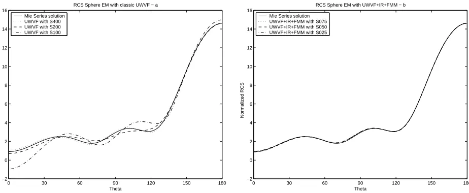
In this section, we compare two codes: the classical UWVF code with a classical ABC of order 0 and the code UWVF+IR+FMM using a 1-level FMM. They were run with the meshes defined in [7]. This led to some comparison figures, Figure 2 (see also the figures 3-4 and 5 in [7]) showing the radar cross section denoted by “RCS” and obtained from the angular dependence of the far field pattern predicted by our codes compared to the exact Mie series.
In Figure 2, we clearly see the impact of the integral representation on the accuracy of the result: the classical UWVF code, as is well known requires a large distance between Γint and Γext. On the other hand, the code UWVF+IR+FMM gives results which fit with the Mie series solution, even with the thin mesh S025.
CPU-time and memory requirements are given in the case of the EM polarization in Table 3. The results are given for the mesh S400 using the classical UWVF code and for the mesh S025 using the code UWVF+IR+FMM. These two cases lead to a comparable accuracy. Even if the curve obtained with S200 using the UWVF code could be acceptable, its accuracy is quite poor in comparison with the one obtained with S025 using the code UWVF+IR+FMM (hence why we compare results for S400 and S025 in Table 3). In the table we use the following notation (the units are the second and the Giga-bytes):
• CPU time:
T00 = precalculation of the matricesC andD.
T0c (resp. T0f) = precalculation of the close (resp. far) interactions related toCe. TD (resp. TC) = one multiplication byD−1 (resp. C) (average).
TCc (resp. TCf) = one multiplication byCe close (resp. far) (average). Tcg = Total CPU time for the solution of the system.
0 30 60 90 120 150 180 −2
0 2 4 6 8 10 12 14 16
Theta
Normalized RCS
RCS Sphere EM with classic UWVF − a
Mie Series solution UWVF with S400 UWVF with S200 UWVF with S100
0 30 60 90 120 150 180
−2 0 2 4 6 8 10 12 14 16
Theta
Normalized RCS
RCS Sphere EM with UWVF+IR+FMM − b
Mie Series solution UWVF+IR+FMM with S075 UWVF+IR+FMM with S050 UWVF+IR+FMM with S025
Figure 2. The EM-polarized RCS as a function of polar coordinateθcomputed using the two codes in the study. Left: results for the classical UWVF code with meshes S400, S200 and S100. Right: results for the code UWVF+IR+FMM with the meshes S025, S050 and S075.
Table 3. Computational costs with UWVF (S400) and UWVF+IR+FMM (S025)
Case T00 T0c T0f TD TC TCc TCf Tcg Nit Ttot mem S400 322 – – 1.54 4.22 – – 971 162 1293 4.8 S025 15.5 394.5 13 0.13 0.4 13.6 10.5 1745 126 2168 2.1
• Nit = Number of iterations for the bi-conjuguate gradient.
• mem = Memory required by the code.
In agreement with the theoretical complexity of the algorithm, since we used the UWVF+IR+FMM on S025 versus the UWVF on S400, the cost of the calculation related to the operatorsDandC strongly decreased by using the new method: This cost is divided by about 10 when the thickness of the meshed domain is divided by 4.33. On the other hand since we have used only the 1-level FMM we expect the cost of computing multiplication by ˜Cto be similar to the cost of the UWVF. We exactly observe these facts. For the code UWVF+IR+FMM, the total CPU time is about 1.7 times the one for the classical UWVF code and the memory cost is about 0.4 times the one for the classical UWVF code. Thus the main gain using the 1-level FMM is a much smaller memory cost. Moreover for the code UWVF+IR+FMM, we generate more uniform meshes with the respect of the average edge-length aroundλ/5. Thus the code UWVF+IR+FMM is more stable regarding the conditioning of the linear system and the number of iterations for the bi-conjuguate gradient solver than the classical UWVF.
4.
Conclusion
References
[1] T. Abboud, J.-C. N´ed´elec and B. Zhou, “Improvement of the Integral Equation Method for High Frequency Problems”, Third international conference on mathematical aspects of wave propagation phenomena, SIAM, pp. 178-187, 1995.
[2] O. Cessenat, Application d’une nouvelle formulation variationnelle aux ´equations d’ondes harmoniques - probl`emes de Helmholtz 2D et de Maxwell 3D, PhD-thesis, Universit´e Paris IX, December 1996.
[3] O. Cessenat and B. Despr´es, “Using Plane Waves as Base Functions for Solving Time Harmonic Equations with the Ultra Weak Variational Formulation”, J. Comput. Acoust., vol. 11, pp. 227-238, 2003.
[4] R. Coifman, V. Rokhlin and S. Wandzura, “The Fast Multipole Method for the Wave Equation: A Pedestrian Prescription”, IEEE Antennas and Propagation Magazine, vol. 35 (3), pp. 7–12, June 1993.
[5] D. Colton and R. Kress, Inverse Acoustic and Electromagnetic Scattering Theory, 2nd ed., Springer Verlag, New York, 1998. [6] E. Darrigrand, “Coupling of Fast Multipole Method and Microlocal Discretization for the 3-D Helmholtz Equation”, J. Comput.
Phys., vol. 181 (1), pp. 126–154, September 2002.
[7] E. Darrigrand and P. Monk, “Coupling of the Ultra-Weak Variational Formulation and an Integral Representation using a Fast Multipole Method in Electromagnetism”, J. Comput. and Applied Math., to appear, available online.
[8] E. Darve, “The Fast Multipole Method: Numerical Implementation”, J. Comput. Phys., vol. 160 (1), pp. 195–240, 2000. [9] C. Hazard and M. Lenoir, “On the Solution of Time-Harmonic Scattering Problems for Maxwell’s Equations”, SIAM J. Math.
Anal., vol. 6, pp. 1597-1630, November 1996.
[10] J. Liu and J.M. Jin, “A Novel Hybridization of Higher Order Finite Element and Boundary Integral Methods for Electromag-netic Scattering and Radiation Problems”, IEEE Trans. Ant. Prop., vol. 49, pp. 1794-1806, December 2001.