The Thirty-Third AAAI Conference on Artificial Intelligence (AAAI-19)
Learning Set Functions with Limited Complementarity
Hanrui Zhang
Computer Science DepartmentDuke University Durham, NC 27705 [email protected]
Abstract
We study PMAC-learning of real-valued set functions with limited complementarity. We prove, to our knowledge, the first nontrivial learnability result for set functions exhibiting complementarity, generalizing Balcan and Harvey’s result for submodular functions. We prove a nearly matching informa-tion theoretical lower bound on the number of samples re-quired, complementing our learnability result. We conduct numerical simulations to show that our algorithm is likely to perform well in practice.
Introduction
A central problem in economics and algorithmic game the-ory is to price items. Intuitively, a seller would like to set the highest price such that the customer would still buy, which requires decent understanding of the customer’s val-uation. When there are multiple items which can be sold in any combination, the valuation is usually modeled as a set function with the items being the ground set. That is, the valuation function of the customer maps each subset of the items to her utility when she gets the subset. To be able to better price the items for maximum profit, one need to learn the customer’s valuation function. Set functions are also used to model influence propogation in social networks (Kempe, Kleinberg, and Tardos 2003), and for solving clus-tering problems (Narasimhan and Bilmes 2007). In all these scenarios, learning the corresponding set function plays an essential part in solving the problem.
There is a rich body of research on learning of set func-tions, e.g. (Balcan and Harvey 2011; Balcan et al. 2012; Lin and Bilmes 2012; Bach and others 2013). All of these re-sults focus on an important class of monotone set functions —complement-freeset functions. Such set functions model the natural property of diminishing returns, and are gener-ally considered much easier to tackle than general monotone set functions. For example, various optimization problems admit efficient constant factor approximations when the set function involved is complement-free or submodular (which is stronger than complement-free) (Nemhauser and Wolsey 1978; Vondr´ak 2008; Feige 2009), while for general mono-tone functions the best possible approximation ratio can be arbitrarily large.
Copyright c2019, Association for the Advancement of Artificial Intelligence (www.aaai.org). All rights reserved.
However, in real-world scenarios, it is common that a val-uation function exhibitslimited complementarity. For exam-ple, a pen is useful only if accompanied by paper to write on. Paper therefore complements pens. This complementar-ity to pens is limited, in the sense that owning items other than paper, like computers, is unlikely to make pens more valuable. So in the above example, complementarity exists only between pens and paper. One significant real-world example of limited complementarity is the spectrum auc-tions, where the rights to use specific bands in specific re-gions are sold. The complementarity there lies in the fact that a buyer would like the same band in neighboring re-gions (say states). Since there are only 50 states, one would naturally cosider the degree of complementarity limited. More motivating everyday examples of limited complemen-tarity can be found in (Feige et al. 2015; Eden et al. 2017; Chen, Teng, and Zhang 2019).
In the past decade, there has been a growing interest in studying set functions with limited complementarity, es-pecially in the combinatorial optimization and algorith-mic game theory communities. In particular, recent results seem to suggest, that there exists smooth transitions from complement-free to completely arbitrary monotone set func-tions, parametrized by the degree of complementarity of the function. The transitions support graceful degrading of the approximation ratio for various combinatorial optimiza-tion tasks (Feige and Izsak 2013; Feldman and Izsak 2014; Feige et al. 2015; Chen, Teng, and Zhang 2019), and the revenue and efficiency (measured by the Price of Anarchy) of well-studied simple protocols for combinatorial auctions (Feige et al. 2015; Feldman et al. 2016; Eden et al. 2017; Chen, Teng, and Zhang 2019).
So one natural question arises:
Is there a way to generalize learnability of complement-free set functions to those with limited complementarity, without incurring too much penalty?
In this paper, based on understanding of the underly-ing combinatorial and statistical structures, we give, to our knowledge, the first nontrivial learnability result for mono-tone set functions with limited complementarity:
Theorem 1 (Main Theorem (Informal)). Restricted to product distributions, there is an efficient algorithm that
func-tion with fixed degree of complementarity.
The above theorem generalizes a central result of (Balcan and Harvey 2011) beyond complement-free functions. We also complement our result by a nearly matching informa-tion theoretical lower bound. We conduct numerical simula-tions to show that our algorithm is likely to perform well in practice.
Define themarginalofSgivenT, denoted byf(S|T), to bef(S|T) :=f(S∪T)−f(T). Throughout the paper, when we refer to a set functionf, unless otherwise specified, we always assume that:
• f has aground set[n] = {1,2, . . . , n}. That is, f maps all subsets of[n], denoted by2[n], to real numbers.
• f is (weakly)monotone. That is, for anyS ⊆ T ⊆ [n],
f(S)≤f(T).
• f is1-Lipschitz. That is, for anyS ⊆ [n]andv ∈ [n],
f(v|S)≤1.
PMAC-Learning
To study learnability of real-valued functions, we use the Probably Mostly Approximately Correct (PMAC) model introduced by Balcan and Harvey in (Balcan and Harvey 2011).
Definition 1(PMAC-Learning (Balcan and Harvey 2011)). LetFbe a family of functions with domain2[n]. We say that
an algorithmAPMAC-learnsF with approximation factor
α, if for any distributionDover2[n], target functionf∗∈ F,
and for any sufficiently smallε≥0, δ≥0,Atakes as input a set of samples{(Si, f∗(Si)}i∈[`]where eachSiis drawn
independently fromD, and outputs a functionf : 2[n] →
R inFthat satisfies
Pr
S1,...,S`∼D
h
Pr
S∼D[f(S)≤f
∗(S)≤α·f(S)]≥1−εi
≥1−δ,
where the number of samples`and the running time ofA
are bothpoly(n,1/ε,1/δ).
In words, the definition says the algorithm succeeds with probability1−δ, upon which it outputs an approximationf
off∗such that with probability1−ε,f∗(S)is within fac-torαoff(S). Note that restricted to Boolean-valued func-tions and letting α = 1, PMAC-learning becomes exactly the classic PAC-learning.
Classes of Set Functions
Numerous classes of complement-free set functions have been proposed and studied, among which the following classes are particularly natural and useful:submodular, frac-tionally subadditive, and subadditive functions. Previous work on learning set functions has been focusing on these classes.
• Submodular. A set functionf is submodular, if for any
v∈[n],S, T ⊆[n],f(v|S∪T)≤f(v|S). The class con-tains essentially all functions with diminishing marginal returns.
• Fractionally subadditive (or XOS). A set function f is fractionally subadditive, if for any S ⊆ [n], k ∈ N,
T1, . . . , Tk ⊆ [n], 0 ≤ α1, . . . , αk ≤ 1, f(S) ≥ P
i∈[k]αif(Ti), as long as the following holds: for any v∈S,P
i∈[k]:v∈Tiαi ≥1. In other words, if{(Ti, αi)}i
form a fractional cover of S, then the weighted sum of
f(Ti)’s is no smaller thanf(S).
• Subadditive (or complement-free).A set functionfis sub-additive, if for anyS, T ⊆[n],f(S) +f(T)≥f(S∪T). It can be shown that every submodular function is fraction-ally subadditive, and every fractionfraction-ally subadditive function is subadditive.
Beyond complement-free functions, several measures of complementarity have been proposed, and the ones particu-larly helpful for our purposes are thesupermodular degree (SD) hierarchyand thesupermodular width (SMW) hierar-chy. They build on the concepts ofpositive dependencyand supermodular setsrespectively.
Definition 2(Positive Dependency (Feige and Izsak 2013)). Given a set function f, an element u ∈ [n] depends pos-itively on v ∈ [n], denoted by u →+ v, if there exists S⊆[n]\ {u}, such thatf(u|S)> f(u|S\ {v}).
Definition 3 (Supermodular Degree Hierarchy (Feige and Izsak 2013)). The supermodular degree of a set functionf, denoted bySD(f), is defined to be
SD(f) := max
u |{v|u→ +v}|.
For anyd ∈ {0,1, . . . , n−1}, a function f is in the first
dlevels of the supermodular degree hierarchy, denoted by
f ∈SD-d, ifSD(f)≤d.
The definitions essentially say, thatudepends positively onvif addingvto some set makes the marginal ofugiven that set strictly larger, and the supermodular degree of f
is then the maximum number of elements on which some particular element positively depends. The degree then nat-urally categorizes functions into hierarchies.
Definition 4 (Supermodular Set (Chen, Teng, and Zhang 2019)). A setT ⊆[n]is a supermodular set w.r.t.f, if there existsv∈[n]andS⊆[n], such that for allT0(T,
f(v|S∪T)> f(v|S∪T0).
Definition 5(Supermodular Width Hierarchy (Chen, Teng, and Zhang 2019)). The supermodular width of a set function
f, denoted bySMW(f), is defined to be
SMW(f) := max{|T| |T is a supermodular set}.
For anyd ∈ {0,1, . . . , n−1}, a function f is in the first
d levels of the supermodular width hierarchy, denoted by
f ∈SMW-d, ifSMW(f)≤d.
That is to say,T is a supermodular set, if given “environ-ment”S, v has a larger marginal given T than given any proper subset ofT, and the supermodular width off is the size of the largest supermodular set.
Proposition 1((Chen, Teng, and Zhang 2019)). For any set function f,SMW(f) ≤ SD(f). Or equivalently, for any
d∈ {0,1, . . . , n−1},SD-d⊆SMW-d.
So theSMWhierarchy is a refinement of theSD hierar-chy. Our results will be established with respect to theSMW hierarchy, and then immediately apply to theSDhierarchy.
Our Results and Techniques
We study PMAC-learning the class of monotone, nonnega-tive,1-Lipschitz set functions with minimum nonzero value 1 inSMW-d ⊇ SD-d. Parameter dhere controls the de-gree of complementarity in these set functions. In particular, whend= 0, we recover the learnability result for submod-ular functions (Balcan and Harvey 2011).
We restrict our investigation of learnability to product dis-tributions for the following reason:under arbitrary distri-butions, every algorithm for PMAC-learning monotone, submodular functions must have approximation factor
˜
Ω(n1/3)1, even if the functions are1-Lipschitz (Balcan and Harvey 2011).Note that the maximum possible value of a normalized monotone1-Lipschitz function isn. In other words, there is no hope for learnability with a decent approx-imation factor when the underlying distribution is arbitrary. While product distributions may appear not entirely satisfac-tory in modeling the real world, we argue that the assump-tion is still to some extent realistic: for example, pawn shops buy items brought to them by different people independently at random, but may sell items in combinations. In general, the assumption holds for any entity that acquires items inde-pendently and bundles them for selling.
Breaking the task down. As observed by Balcan and Har-vey (Balcan and HarHar-vey 2011), the task of learning submod-ular set functions can be divided into two parts: learning0’s of the function, and learning the distribution of positive val-ues. We observe a similar phenomenon for functions with complementarityd. We therefore break the task down into two parts, with the first subtask being intrinsically combina-torial, and the second subtask statistical. The plan is to estab-lish learnability for both subtasks respectively, and combine them into learnability of monotone, nonnegative functions with complementarityd.
The combinatorial subtask. In the combinatorial sub-task, the goal is to PAC-learn monotone Boolean-valued functions inSMW-d ⊇ SD-d. By observing the combina-torial structure of a Boolean-valuedSMW-dfunction, we show that all information of the function is encoded in sets of size not exceedingd+ 1. This observation immediately leads to an algorithm that PAC-learns these functions using
O(nd+1log(n/δ)/ε)samples.
Hardness of learning Boolean-valued functions. We show that, somewhat surprisingly, the combinatorial sub-task is the hardcore of learning nonnegative set functions
1˜
Ωhides a polylog factor.
with complementarityd. Specifically, we prove that any al-gorithm that PAC-learns these functions requires Ω(˜ nd+1)
samples, whereΩ˜hides a polylog factor. Our proof proceeds by constructing a random functionf, where the values off
at sets of size smaller thand+ 1are0, and the values at sets of size exactlyd+ 1are i.i.d., drawn uniformly at random from{0,1}. We further fix the product distribution, such that each elementi∈[n]appears with probability(d+ 1)/n. We show, that it is hard to learn the values at sets of sized+ 1 without enough samples. Then, since with constant proba-bility a sample is of size exactlyd+ 1, the algorithm must output a wrong value with constant probability.
The statistical subtask. In the statistical subtask, the goal is to PMAC-learn monotone positive functions in SMW-d ⊇ SD-d. We show that, unlike Boolean-valued functions, learning positive functions with constant comple-mentarity with approximation factorO(1/ε)requires only
O(n2log(1/δ))samples. This bound matches the result for
submodular functions up to a constant factor(d+ 1)2. The proof proceeds essentially by leveraging the strong con-centration properties we establish. Generalizing Balcan and Harvey’s result for submodular functions (Balcan and Har-vey 2011), we show, that under product distributions, the value of the function converges sharply around the median value, and the mean cannot be too far away from the median. It follows that with high probability, with enough samples, the empirical mean is a good approximation of the value at a random set.
Putting it together. With algorithms for Boolean-valued and positive functions at hand, it is natural to put them to-gether, in the hope that the combination takes care of both subtasks. We show that this is indeed what happens — with approximation factor O(log(1/ε)), the combination of the two algorithms PMAC-learns nonnegative functions with complementaritydusing
O(n2log(1/δ) +nd+1log(n/δ)/ε)
samples, where the first term is for positive values, and the second is for0’s. While it may seem weird that samples for learning0’s dominate the total number of samples, we note that the lower bound for learning Boolean-valued functions also applies for nonnegative functions, since the latter sub-sume the former as a subclass. It follows that the dependency inn in our upper bound is almost tight. We further show, that when the empirical mean is large enough, the number of samples needed becomes significantly smaller. This is be-cause we no longer need to learn the0’s, since concentration bounds guarantee that the probability of a0is negligible.
Additional Related Work
Du et al. (Du et al. 2014) and
func-tions (Badanidiyuru et al. 2012; Devanur et al. 2013; Cohavi and Dobzinski 2017). There are a number of results on testing submodularity (Seshadhri and Vondr´ak 2014; Blais and Bommireddi 2017).
Beside theSDand theSMW hierarchies, there are sev-eral other measures of complementarity, among which two most useful ones are Maximum-over-Positive-Hypergraphs (MPH) (Feige et al. 2015) and its variant, Maximum-over-Positive-Supermodular (MPS) (Feldman et al. 2016).
The Combinatorial Subtask: Learning
Boolean-Valued Functions
In this section we consider PAC-learning ofF∗d, the class of
monotone Boolean-valued functions inSMW-d⊇SD-d.d
can be viewed as a constant measuring the degree of com-plementarity. As we will see, PAC-learningF∗
d is the
infor-mation theoretical hard core of PMAC-learning set functions with limited complementarity.
First we characterize the structure of0’s of a set function inF∗
d. We sayS ⊆[n]is azero set(w.r.t.f) iff(S) = 0.
Unlike submodular functions, whose system of zero sets is closed downward and under union, a function inF∗
d may
have zero sets with notably more complicated structure. In particular, even iff(S) = f(T) = 0, it is not necessarily true thatf(S∪T) = 0. To efficiently learnF∗
d, we leverage
the following succinct representation of its members’ zero sets:
Lemma 1(Structure of Zero Sets). For a monotone set func-tion f ∈ SMW-d, f(S) = 0 iff for all T ⊆ S where
|T| ≤d+ 1,f(T) = 0.
In other words, all information aboutf’s zero sets is en-coded in values offat sets with size no larger thand+ 1. As a result, to distinguish0’s off, we only need to keep track of its zero sets of constant size. This characterization leads directly to Algorithm 1.
Proof of Lemma 1. By monotonicity, clearly if f(S) = 0 then for anyT ⊆ S,f(T) = 0. We now prove the other direction. Suppose for allT ⊆Swhere|T| ≤d+1,f(T) = 0. We assumef(S)>0and show a contradiction. LetS0⊆ S be a subset of S with the smallest cardinality such that
f(S0) > 0. Clearly |S0| ≥ d+ 2, and for any T
( S0,
f(T) = 0. Letvbe any element inS0.
0< f(S0) =f(v|S0\ {v})
≤max{f(v|T)|T ⊆S0\ {v},|T| ≤d} ≤max{f(T)|T ⊆S0,|T| ≤d+ 1}
= 0.
Theorem 2 (PAC-Learnability of Boolean-Valued Func-tions). Restricted to product distributions, for any suffi-ciently smallε > 0 and δ > 0, Algorithm 1 PAC-learns
F∗
d with parameters(ε, δ). The number of samples is ` =
10(d+ 1)nd+1log(n/δ)/ε.
Algorithm 1:An algorithm that PAC-learns monotone Boolean-valued functions with limited complementarity.
Input : `samples{(Si, f∗(Si))}i∈[`]from a product
distributionD.
Output: with high probability, an approximately correct estimationfoff∗.
LetL ← ∅. fori∈[`]do
iff∗(Si) = 0, and there exists a subsetT ofSiwith |T| ≤d+ 1, such thatT /∈ Lthen
forEvery subsetU ofSiwith|U| ≤d+ 1do
LetL ← L ∪ {U}.
Outputf, wheref(S) = 0iff for any subsetTofS
with|T| ≤d+ 1,T ∈ L.
Proof of Theorem 2. We prove a slightly stronger but essen-tially similar claim, that with probability1−1
2δ, the
algo-rithm succeeds, and the probability of not recognizing a0is at most 12ε. First note that the familyLcontains only sets of size no larger thand+ 1, so its cardinality cannot exceed
X
0≤i≤d+1 n
i
≤ X
0≤i≤d+1 ni= n
d+2−1
n−1 ≤2n
d+1.
Every time we fail to recognize a0, the size ofLgrows by at least 1. So this can happen at most 2nd+1 times. As
long as there is a12εprobability that we fail to recognize a0, on average we encounter such a sample within2εsteps. And in fact, in8(d+ 1) log(n/δ)/εsteps, the probability of no update is
1−1
2ε
8(d+1) log(n/δ)/ε < δ
4nd+1.
If after some update, the probability that we fail to recog-nize a0drops below 12ε, the conditions of the theorem are already met. Otherwise, after all updates toL, there is still a 12 probability that we encounter a0that cannot be recog-nized, and the algorithm fails.
We now bound the probability of such a global failure. A union bound over each update immediately gives that after
` >10(d+ 1)nd+1log(n/δ)/ε >8(d+ 1)nd+1log(n/δ)/ε
steps, the probability that we have not finished the2nd+1
updates is at most δ2. This implies that after seeing all sam-ples, with probability at least1−δ
2 the algorithm succeeds,
in which case the probability thatLfails to recognize a0of
f∗(X)is at most 12ε.
As shown by Balcan and Harvey, PAC-learning Boolean-Valued submodular functions (i.e.F∗
0) under product
distri-butions requires only O(nlog(n/δ)/ε) samples. One may question if thend+1factor forF∗
d is necessary. We prove the
following lower bound, showing that such a factor is neces-sary for any algorithm that PAC-learnsF∗
Theorem 3(LearningF∗
dRequires Many Samples). Fix any δ >0,d∈N, for large enoughnandε < 14
1 e
d+1
, any al-gorithm that PAC-learnsF∗
d with parameters(ε, δ)under a
product distribution over2[n]requiresΩ(nd+0.99)samples.
0.99can be replaced by any number smaller than1.
Proof sketch. Considerf∗ : 2[n] → {0,1}drawn from the
following distribution:
• ForSwhere|S| ≤d,f∗(S) = 0.
• ForSwhere|S|=d+ 1,f∗(S) = 0w.p.0.5. Otherwise
f(S) = 1.
• ForS where|S| > d+ 1,f∗(S) = 0 if for allT ⊆ S
where|T|=d+ 1,f∗(T) = 0. Otherwisef∗(S) = 1.
It is easy to check that any such function is inSMW-d. Consider a product distribution over2[n], where each
ele-menti ∈[n]appears with probability(d+ 1)/n. One may show that under this distrbution, with constant probability a random set has size preciselyd+ 1. Therefore, to learnf∗, any algorithm must learn correctly the values of most sets of sized+ 1. There are aboutnd+1such sets in total.
On the other hand, standard concentration bounds guar-antee that a sample set is almost always not too large. In fact, with high probability, all the sample sets have cardinal-ity at mostO(dlogn). As a result, onlyO((logn)d+1)sets
of sized+ 1can be subsets of a sample set. Conditioned on the event that all sample sets are not too large, since each sample set can only reveal values off∗ at the critical sets
it contains, with one sample, the algorithm learns at most
O((logn)d+1)values at critical sets. So with relatively few
samples, almost always the algorithm fails to learn the val-ues at most critical sets, and therefore does not have enough information aboutf∗. The lower bound follows.
The Statistical Subtask: Learning Positive
Functions
In this section we consider learning real-valued functions in
F+
d, the family of monotone, positive,1-Lipschitz set
func-tions with minimum nonzero value1 inSMW-d ⊇ SD-d. we note that these are standard regularity assumptions for PMAC-learning (Balcan and Harvey 2011).
Concentration with Limited Complementarity
Our most powerful tool for learningFd+is a strong concen-tration bound, generalizing Balcan and Harvey’s result for submodular functions (Balcan and Harvey 2011).Lemma 2. Letf ∈ SMW-dbe a monotone, nonnegative, 1-Lipschitz set function with minimum nonzero value1. Let
Dbe a product distribution over2[n]. For anyb, t≥0,
Pr
X∼D
h
f(X)≤b−t√bi·Pr[f(X)≥b]
≤exp(−t2/4(d+ 1)2).
The lemma immediately gives concentration around the median. LetMed(Z)denote the median of real-valued ran-dom variableZ. We have:
Corollary 1(Concentration Around the Median). Letf ∈
SMW-dbe a monotone, nonnegative,1-Lipschitz set func-tion with minimum nonzero value1. LetDbe a product dis-tribution over2[n]. For anyt≥0andX∼ D,
Pr
X∼D
h
f(X)−Med(f(X))≥tpMed(f(X))i
≤2 exp(−t2/4(d+ 1)2),
(1)
and
Pr
X∼D
h
Med(f(X))−f(X)≥tpMed(f(X))i
≤2 exp(−t2/4(d+ 1)2). (2)
Proof. Letb=Med(X)in Lemma 2. We get
Prhf(X)≤Med(f(X))−tpMed(f(X))i
· Pr[f(X)≥Med(f(X))]
≤ exp(−t2/4(d+ 1)2).
By definition of medians, we have
Pr[f(X)≤Med(f(X))]≥1/2.
So,
Prhf(X)≤Med(f(X))−tpMed(f(X))i
≤ exp(−t2/4(d+ 1)2)/Pr[f(X)≤Med(f(X))]
≤2 exp(−t2/4(d+ 1)2).
Similarly, lettingb=Med(X) +tpMed(f(X)), we get
Prhf(X)≥Med(f(X)) +tpMed(f(X))i
≤2 exp(−t2/4(d+ 1)2).
We further show that the above concentration bounds around the median can be translated to concentration around the mean, by arguing that the mean is always close to the median:
Lemma 3. Letf ∈ SMW-dbe a monotone, nonnegative, 1-Lipschitz set function with minimum nonzero value1. Let
Dbe a product distribution over2[n]. ForX ∼ D,
E[f(X)]≥ 1
2Med(f(X)),
E[f(X)]≤Med(f(X)) + 8(d+ 1)pMed(f(X)).
Intuitively, these bounds suggest that set functions with limited complementarity, in spite of much weaker separabil-ity conditions, have similar concentration behavior to con-centration of additive set functions from Hoeffding style ar-guments.
We note that similar results can be obtained through con-centration of self-bounding functions. See, e.g., (Boucheron, Lugosi, and Bousquet 2004; Vondr´ak 2010). In particular, one may show that every monotone 1-Lipschitz SMW-d
Algorithm 2: An algorithm that PMAC-learns mono-tone positive functions with limited complementarity.
Input : `samples{(Si, f∗(Si))}i∈[`]from a product
distributionD.
Output: with high probability, a mostly approximately correct estimationf off∗.
Letµ← 1 `
P
i∈[`]f∗(Si).
ifµ≥1000(d+ 1)2log(1/ε)then
Outputf(S) =10µ.
else
Outputf(S) = 1.
PMAC-Learning Algorithm for Positive Functions
Equipped with these strong concentration bounds, we are ready to present the PMAC-learning algorithm forF+d .
Theorem 4 (PMAC-Learnability of Positive Functions). Restricted to product distributions, for any sufficiently small
ε >0andδ >0, Algorithm 2 PMAC-learnsF+ d with: • parameters(ε, δ),
• approximation factorα=O((d+ 1)2log(1/ε)), and • number of samples`= 10n2log(1/δ).
WhenE[f∗(X)]≥c(d+ 1)2log(1/ε)for sufficiently large c, the approximation factor improves to20.
Proof sketch. According to Hoeffding’s inequality, with high probability the empirical meanµ is an estimation of E[f∗(X)]with constant additive error. We then proceed by two cases:
1. µ is large enough. This means E[f∗(X)], and by Lemma 3,Med(f∗(X)), are also large enough. Soµis multiplicatively a good estimation ofMed(f∗(X)), and Corollary 1 therefore applies approximately aroundµ. It is then sufficient to output a constant fraction ofµ. The approximation factorαin this case is a constant. 2. µ is relatively small. This means E[f∗(X)], and by
Lemma 3,Med(f∗(X)), are relatively small. It follows from Corollary 1 that with high probability, f∗(X) is
close enough to1. It is then sufficient to output1, since
f∗ ∈ F+
d is positive. The approximation factorαin this
case isO((d+ 1)2log(1/ε)).
Putting Everything Together: Learning
General Functions
Now we handle the general case: PMAC-learning Fd, the
family of monotone, nonnegative,1-Lipschitz set functions with minimum nonzero value1 inSMW-d ⊇SD-d. With Theorems 2 and 4 at hand, it is natural to combine Algo-rithms 1 and 2, in the hope of taking care of both the combi-natorial and the statistical aspects of the problem simultane-ously. We prove, not too surprisingly, that such a combina-tion PMAC-learnsFd.
Algorithm 3: An algorithm that PMAC-learns mono-tone nonnegative functions with limited complementar-ity.
Input : `samples{(Si, f∗(Si))}i∈[`]from a product
distributionD.
Output: with high probability, a mostly approximately correct estimationfoff∗.
Letµ← 1 `
P
i∈[`]f∗(Si).
ifµ≥1000(d+ 1)2log(1/ε)then Outputf(S) = 10µ.
else
LetL ← ∅. fori∈[`]do
iff∗(S
i) = 0, and there exists a subsetTofSi
with|T| ≤d+ 1, such thatT /∈ Lthen forEvery subsetU ofSiwith|U| ≤d+ 1
do
LetL ← L ∪ {U}.
Outputf, wheref(S) = 0if for any subsetT ofS
with|T| ≤d+ 1,T ∈ L, andf(S) = 1otherwise.
Theorem 5 (PMAC-Learnability of General Functions). Restricted to product distributions, for sufficiently smallε >
0andδ >0, Algorithm 3 PMAC-learnsFdwith:
• parameters(ε, δ),
• approximation factorα=O((d+ 1)2log(1/ε)), and • number of samples ` = 10n2log(1/δ) + 10(d +
1)nd+1log(n/δ)/ε.
WhenE[f∗(X)]≥c(d+ 1)2log(1/ε)for sufficiently large
c, the approximation factor improves to20, and the number of samples improves to`= 10n2log(1/δ).
Proof sketch. Again, consider the two cases:
1. µ is large enough. Lemma 3 and Corollary 1 establish the same strong concentration aroundµ, so it is sufficient to output a constant fraction ofµ. In this case we do not need samples in the next phase, so the number of samples needed is10n2log(1/δ). And for similar reasons, the ap-proximation factor is20.
2. µis relatively small. Becausef∗is now nonnegative, we need to consider0’s off∗. When our estimation is wrong, it can be either (1) f(S) = 1 andf∗(S) = 0, or (2)
f(S) = 1 and f∗(S) is too large. By adapting
Theo-rem 2 we can show that situation (1) happens with prob-ability at most 12ε, and by Theorem 4, situation (2) hap-pens with probability at most12ε. The overall probability of a wrong estimation is at mostε. In this case we need all
`= 10n2log(1/δ)+10(d+1)nd+1log(n/δ)/εsamples,
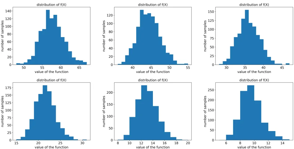
Figure 1: Distributions off(X)when the degree of complementarity is0,1,2,5,10, and15.
Note that since Fd subsumes Fd∗, Theorem 3 directly
implies the same information theoretical lower bound for PMAC-learningFd, complementing Theorem 5. Formally:
Corollary 2 (Learning Fd Requires Many Samples). Fix
anyδ >0,d ∈N, for large enoughnandε < 14 1 e
d+1
, any algorithm that PAC-learns Fd with parameters (ε, δ)
under a product distribution over 2[n], with any
approxi-mation factor, requiresω(nd+0.99)samples.0.99can be re-placed by any number smaller than1.
We note again, that since theSMW hierarchy is strictly more expressive than theSDhierarchy (Proposition 1), all our learnability results for functions inF∗
d,F +
d andFd
ap-ply to functions with the same set of requirements but with SMW-dreplaced bySD-d.
Numerical Simulations
We conduct numerical simulations to investigate the empir-ical concentration of set functions with limited complemen-tarity. Unfortunately, there is no efficient way known to gen-erate set functions inSMW-dorSD-d. Instead, we sample functions from the Maximum-over-Positive-Hypergraphs (MPH) hierarchy (Feige et al. 2015), which is another well-known measure of complementarity. It has also been used to study the equilibrium behavior of agents in certain auc-tion protocols (Feige et al. 2015). In some sense, the exper-imental results with MPH functions should be considered a complement to our theoretic results, as it sheds light on the statistical behavior of functions considered to have lim-ited complementarity according to another commonly used measure, even if Theorem 5 does not always provide strong guarantees for them.
The MPH hierarchy builds on the concept ofhypergraphs. Roughly speaking, a hypergraph can be viewed as a set func-tion, where the value of a set is the sum of the weights of hy-peredges that the set contains. A function is inMPH-(d+1), if there exists a finite number of hypergraphs containing only positively weighted hyperedges of size at most(d+ 1), such that the value of the function at any set is the maximum value of the set in these hypergraphs.MPH-0is exactly the class of functions that are fractionally subadditive.
In our experiments, we fix the cardinality of the ground set to be n = 1000and the number of hypergraphs to be 10. In each hypergraph, we choose uniformly at random100 disjoint sets of size chosen from{1,2, . . . , d+ 1}uniformly at random. For each degree of complementarityd, we sam-ple a functionfinMPH-din the way described above, draw 1000sample sets where each element appears with probabil-ity0.5, and plot the empirical distribution off(X).
Acknowledgements
We are thankful for support from NSF under awards IIS-1814056 and IIS-1527434. We also thank Wei Chen, Shang-Hua Teng, and anonymous reviewers for helpful feedback.
References
Bach, F., et al. 2013. Learning with submodular functions: A convex optimization perspective.Foundations and TrendsR in Machine Learning6(2-3):145–373.
Badanidiyuru, A.; Dobzinski, S.; Fu, H.; Kleinberg, R.; Nisan, N.; and Roughgarden, T. 2012. Sketching valua-tion funcvalua-tions. InProceedings of the twenty-third annual ACM-SIAM symposium on Discrete Algorithms, 1025–1035. Society for Industrial and Applied Mathematics.
Balcan, M.-F., and Harvey, N. J. 2011. Learning submodular functions. In Proceedings of the forty-third annual ACM symposium on Theory of computing, 793–802. ACM. Balcan, M. F.; Constantin, F.; Iwata, S.; and Wang, L. 2012. Learning valuation functions. In Conference on Learning Theory, 4–1.
Blais, E., and Bommireddi, A. 2017. Testing submod-ularity and other properties of valuation functions. In LIPIcs-Leibniz International Proceedings in Informatics, volume 67. Schloss Dagstuhl-Leibniz-Zentrum fuer Infor-matik.
Boucheron, S.; Lugosi, G.; and Bousquet, O. 2004. Con-centration inequalities. InAdvanced Lectures on Machine Learning. Springer. 208–240.
Chen, W.; Teng, S.-H.; and Zhang, H. 2019. Capturing Com-plementarity in Set Functions by Going Beyond Submodu-larity/Subadditivity. InProceedings of the 10th conference on Innovations in Theoretical Computer Science.
Cohavi, K., and Dobzinski, S. 2017. Faster and simpler sketches of valuation functions. ACM Transactions on Al-gorithms (TALG)13(3):30.
Devanur, N. R.; Dughmi, S.; Schwartz, R.; Sharma, A.; and Singh, M. 2013. On the approximation of submodular func-tions.arXiv preprint arXiv:1304.4948.
Du, N.; Liang, Y.; Balcan, M.; and Song, L. 2014. Influence function learning in information diffusion networks. In In-ternational Conference on Machine Learning, 2016–2024. Eden, A.; Feldman, M.; Friedler, O.; Talgam-Cohen, I.; and Weinberg, S. M. 2017. A simple and approximately optimal mechanism for a buyer with complements. InProceedings of the 2017 ACM Conference on Economics and Computation, 323–323. ACM.
Feige, U., and Izsak, R. 2013. Welfare maximization and the supermodular degree. InProceedings of the 4th conference on Innovations in Theoretical Computer Science, 247–256. ACM.
Feige, U.; Feldman, M.; Immorlica, N.; Izsak, R.; Lucier, B.; and Syrgkanis, V. 2015. A unifying hierarchy of valuations with complements and substitutes. InAAAI, 872–878. Feige, U. 2009. On maximizing welfare when utility functions are subadditive. SIAM Journal on Computing 39(1):122–142.
Feldman, M., and Izsak, R. 2014. Constrained monotone function maximization and the supermodular degree. Ap-proximation, Randomization, and Combinatorial Optimiza-tion. Algorithms and Techniques160.
Feldman, M.; Friedler, O.; Morgenstern, J.; and Reiner, G. 2016. Simple mechanisms for agents with complements. InProceedings of the 2016 ACM Conference on Economics and Computation, 251–267. ACM.
Kempe, D.; Kleinberg, J.; and Tardos, ´E. 2003. Maximizing the spread of influence through a social network. In Proceed-ings of the ninth ACM SIGKDD international conference on Knowledge discovery and data mining, 137–146. ACM. Lin, H., and Bilmes, J. 2012. Learning mixtures of sub-modular shells with application to document summarization. InProceedings of the Twenty-Eighth Conference on Uncer-tainty in Artificial Intelligence, 479–490. AUAI Press. Narasimhan, M., and Bilmes, J. A. 2007. Local search for balanced submodular clusterings. InIJCAI, 981–986. Narasimhan, H.; Parkes, D. C.; and Singer, Y. 2015. Learn-ability of influence in networks. InAdvances in Neural In-formation Processing Systems, 3186–3194.
Nemhauser, G. L., and Wolsey, L. A. 1978. Best algorithms for approximating the maximum of a submodular set func-tion. Mathematics of operations research3(3):177–188. Seshadhri, C., and Vondr´ak, J. 2014. Is submodularity testable? Algorithmica69(1):1–25.
Vondr´ak, J. 2008. Optimal approximation for the submodu-lar welfare problem in the value oracle model. In Proceed-ings of the fortieth annual ACM symposium on Theory of computing, 67–74. ACM.