Network Adaptive Behaviour and its Optimal Performance

(1)

Annals. Computer Science Series. 11 Tome 2 Fasc. – 2013

N

E

T

W

O

R

K

A

D

A

P

T

I

V

E

B

E

H

A

V

I

O

U

R

A

N

D

I

T

S

O

P

T

I

M

A

L

P

E

R

F

O

R

M

A

N

C

E

A

k

h

i

g

b

e

–

M

u

d

u

T

h

u

r

s

d

a

y

E

h

i

s

Department of Computer Science, Federal University of Agriculture Abeokuta. Nigeria.

ABSTRACT: Adaptation is a fundamental characteristic of living organisms since they attempt to maintain physiological equilibr ium in the midst of changing environmental conditions. An approach to the design of adaptive systems is to consider the adaptive aspects of human or animal behavior and to develop systems which behave somewhat analogously. Hence, good performance of networks requires the design of effective control strategies that are capable of rapid adaptation to new circumstances. We designed a frame work algorithms to carry out real – time network traffic, capture the traffic through a sample run of this algorithms. The level of performance is measured by the mean value of temperatures using an ANOVA statistics and the measurements were used to display a performance graph. It is observed that network performance suffers starvation at various levels of environmental changes, and this affects Quality of Service. Our approach is adjudged an efficient approach for network adaptive measures.

KEYWORDS: adaptation, performance, optimal, behavior, environmental and temperature

1. INTRODUCTION

Adaptation is a fundamental characteristic of living organisms since they attempt to maintain physiological equilibrium in the midst of changing environmental conditions. All organisms have adaptations that help them survive and thrive. Some adaptations are structural (anatomical), behavioral or physiological. Anatomical adaptations are physical features of organisms like the fur on a bear or the shape of an animal. Behavioral adaptations are the things organisms do to survive, they can be inherited or learnt and it includes tools, language and swarming behavior. [Dob08]. Autonomic communications systems must demonstrate behavior that remains correct under a range of environmental conditions. An approach to the design of adaptive systems is then to consider the adaptive aspects of human or anima l behavior and to develop systems which behave somewhat analogously. In order to gain confidence that a system will behave as intended, it is advantageous to have a formal description of the expected behavior that can be analyzed and tested for compliance with different stimuli [CZ10]. In this paper, we propose an adaptive systems perspective on a recently proposed formal analytical model of network performance. We suggest how this can be used to study the adaptive behavior of systems and to

ensure that their adaptations maintain desired properties. If system parameters vary widely according to environmental changes, however, then the control system may exhibit satisfactory response for one environmenta l condition but may fail to provide satisfactory performance under other conditions. In such case, large variations of system parameters may cause instability. Generally, all mathematically tractable performance indexes have one serious drawback in common, though they specify the cost of system operation in terms of error and energy, they do not give us information about the transient response characteristics of the system [Oga86]. Thus a system that is designed to operate optimally may have undesirable tra nsient characteristics or may even be unstable. On account of these factors, conventional analytical modeling of networks becomes a tedious task. Yet, the good performance of networks requires the design of effective control strategies that are capable of rapid adaptation to new circumstances. This implies not only a lot of processing time, but also a huge amount of memory to maintain the past records. We therefore, need to have an efficient learning paradigm that economizes both time and space of network management resources [G+11]. Human operator recognizes familiar inputs and can use his past learned experiences in order to react in an optima l manner. A learning system is a higher level system to human operator in any adaptive conditions, it is a system which is capable of recognizing the familiar features and patterns of a situation and which uses its past learned experiences in building an optima l fashion.

2. LITERATURE REVIEW

(2)

oscillates or fail to deliver a feasible network configuration. Policies themselves need to be managed and adaptation can itself be specified and enforced by other policies. [BLV98] proposed network adaptive TCP slow starter to provide a mechanism for performing the transfer of small files much more efficiently than is currently done with TCP. The work here relied on previous network performance history as well as the size of the data in an effort to speed up the file transfer. There are a number of things to be improved upon in this work. First of it all, is a lot of the parameters for the round trip times are untested. Secondly, many assumptions have been made for the purpose of simulation, going from well connected local domain to another across a WAN of unknown characteristics [W+06]. The rapid growth of wireless communications networks has put tremendous pressure on network‟s resources. As a result, efficient adaptive systems are required for effective resource management which constitutes a challenging task [MP13].

3. METHODOLOGY

We designed a framework algorithms called Packet Monitor Algorithms (see figure 1) to carry out a real time network management analysis. Traffic is captured through a sample run of this algorithm displayed in figure 2. The output window is then processed into a sequence of M traffic length, the sequence of length n (M) = 30 is again subdivided into three segments



g g and g

1

,

2

.

3



respectively.

 

1

10,

 

2

10. .

 

3

10 n g



n g



and n g



. Analysis of Variance (ANOVA) is used here to test the designed hypothesis, the data in figure 2 shows the data generated, as



i of units of performance rate when the process was operating at each of the three atmospheric temperature levels. Test of significant used is





0.05

. The level of performance is measured by the mean value and

i

X indicates the observed traffic mean at level i where i1, 2.and.3corresponding to temperatures

0 0 0

68 F,72 F and. .76 Frespectively. There is a certain amount of variations among these means, since sample means do not necessarily repeat when repeated samples are taken from a population, some variations can be expected .The question here is; Is this variations among the Xi „s due to chance or is it due to a difference in the traffic rate at each temperature level? The null hypothesis that we test is: (H0:



68



72



76). That is, the true

performance mean is the same at each temperature

tested. In other words, the temperature does not have a sign ificant effec t on the rate of performance. And the alternative to this is:



H

_a

:



₆₈





₇₂





₇₆



, not all means are equal. Thus we shall reject the null hypothesis if the data show that one or more of the means is significantly different from the others. The decision to reject or fail to reject H0 will be made using the F –

distribution and the F – test statistics. That is, we will compare the calculated value of

F F

,

*, to a one tailed critical value of F obtained from statistical table of appendix G [Joh76].

3.1. Packet Monito r Algo rithms

(A) Alg orithm for Port Sca nning

Step 1: Variable Declaration

Decla re variables for storing IP Address and host name and set them to null

Step 2: Input

2.1 En ter va lue of Ho st na me (o r IP Address)

Step3: Scanning

3.1 Declare variab le port = 0 3.2 Declare initia l port = va lue. 3.3 Declare fina l port = va lue.

3.4 Check if the port is available between initia l port and fina l port.

3.5 incremen t port by 1

3.6 Repea t step 3.4 up to fina l port. Step4: Disp lay

4.1 Display a ll the active po rts in GUI forma t

(B) Algo rith m for packet capturing

Step 1: Obta ining the list of netwo rk interfaces 1.1 Crea te a va riab le array of devices 1.2 Detect n etwork interfaces present in user

1.3 Store the above list in devices va riab le. Step 2: Disp laying the list of network interfaces Decla re loop counter in teger variable i and initia lize to 0

Wh ile the value of i is less than the length of the array of devices, do S tep 2.3

Print ou t the na me and descrip tion of the cap tured Network Interface.

Step 3: Open the network interface.

Decla re in teger variable J and initia lize to zero (J=0 )

Wh ile J < leng th of array of devices, Go to S tep 3.3 else Goto S tep 3.7

Check if the network interface at Jth index nu mber in devices a rray is selected. If yes go to S tep 3.6 else go to S tep 3.4

(3)

Open the selected network in terface i.e. Network Interface a t Jth index, then Go to S tep 4

Disp lay that the network interface has no t yet been selected by the u ser. he user. Go to Step 8

Step 4: Capture packets fro m the network interface Is th e menu bu tton of stop capture packet

selected? If yes go to Step 3.8 else go to Step 4.2 Capture the upco ming single pa cket fro m the netwo rk

Disp lay the cap tured packet by going to S tep 5 Step 5: Disp lay the cap tured packet to the user in proper GUI forma t.

Detect user' menu cho ice of the forma t in wh ich captured packet's to be d isp layed

Analyze the packet. Disp lay in Hexadecimal forma t

Goto S tep 6 to save the pa ckets to a temporary file Go back to Step 4.1

Step 6: Save captured packets into a file 6.1 Crea te a tempo rary file say

6.2 Save captu red packets in to the opened file

6.3 Go back to S tep 5.4

Step 7: Close all the open netwo rk interface 7.1 Delete the tempo rary file. 7.2 Clo se the network in terface. Step 8: End

Fig ure 1: packet mo nito r algo rithm

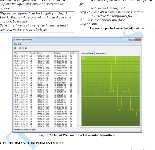
Figure 2: Output Window of Packet monitor Algorithms

4. PERFORMANCE IMPLEMENTATION

Temp level

 

Xi

Replicate (j) Row

 

T

i

Mean

 

Xi

1 2 3 4 5 6 7 8 9 10

680F 161 161 161 161 328 161 161 161 161 239

720F 239 328 202 202 213 78 78 78 78 78

760F 78 161 161 161 161 161 161 161 161 161

Figure 3: Sequence of Data from the Output window

Before performing the calculations on these numbers, let‟s code the data by dividing each data shown in the preceding table by 20. Since ANOVA technique use only measures of variation in the decision making

(4)

Temp (i)

Replication(j) Row

 

T

i

Mean

X

1 2 3 4 5 6 7 8 9 10

680F 8.05 8.05 8.05 8.05 16.4 8.05 8.05 8.05 8.05 11.95 92.75 9.28 720F 11.95 16.4 10.1 10.1 10.65 3.9 3.9 3.9 3.9 3.9 78.7 7.8 760F 3.9 8.05 8.05 8.05 8.05 8.05 8.05 8.05 8.05 8.05 76.35 7.6

Figure 4: A coded Sequence of Data from the Output Window

The analysis of variance (ANOVA) procedure will separate the variations among the entire set of data into two categories. This separation is accomplished by first working the numerator of the fraction that is

used to define sample variance

2 2 1

(

)

1

n i i

X

S

n











. This numerator is called sum of squares:

Sum of squares = 2

1 ( ) n i i X X  



(1)





2 2 1 1 n i n i i i X SS total X

n        









(2)

The SS (total) for our illustration is now found using formula (2). 2 1 2322.95 n i i X  



and

2 1

61, 404.84

n i i

X







_











Thus

SS total







? must now be separated into two parts, sum of squares, SS(temp), due to the temperature levels, and sum of squares, SS(error), due to experimental error of replication. The sum of SS (temp) and SS(error) = SS(total), hence this splitting is often referred to as partitioning.





2 2 1 ( ) n i i i X T SS factor c n       









(3)

where Tirow totals and C are the number of replicates.

 

2

20625.575 i T 



and





 

2 2 1 15.76 n i i i X T SS temp c n        









The sum of squares SS (error), which measures the variation within the rows, is found by use of:





 

2 2 1 i n i i T SS error X

c









(4)

The SS(error) for our illustration is found by use of formula (4)

For convenience we shall use an ANOVA table to record the sum of squares and organize the rest of

the

calculations. The degree of freedom, df,

associated with each of the three rows are

determined as follows:

SS error







260.4

1. df(temp) is I less than the number of levels at

which the factor is tested:





1 df temp

 

r

(5)

2. df(total) is 1 less than the total number of

pieces of data:





1 df total

 

n

(6)

3. df(error) is the sum of the degree of freedom

for all the rows. Each row has c-1 degrees of

freedom; therefore:



 

1 

df error



r c



(7)

The sums of squares and the degrees of freedom

must both check. That is

SS(temp) + SS(error) = SS(total)

.and.

SS(temp)+ df(error) = df(total)

(5)

Source SS df MS

Temp 15.76 2 7.9

Error 260.4 27 9.6

Total 275.8 29

Figure 5: ANOVA table

df(temp) = 3 -1 = 2, df (error) = r (c-1) = 27 and

df( total) = n -1 = 30 – 1 = 29





SS temp

_





_

7.9

MS temp

df temp

 

MS(temp) by MS(error).

The hypothesis test is now completed, using the two mean squares as measures of variance. The calculated value of the test statistics F, F* is found by dividing





. .





.

MS temp by MS error









*

0.78

MS temp F

MS error

 

The decision to reject or fail to reject H0 will be

made by comparing this calculated value of

*

, 0.78

F F  to a one tailed critical value of “F” obtained from table 8a of appendix G [Joh76]. Fail to reject H0 .

0.05



2,27,0.05



3.39 F



Figure 6: Showing the Critical Region

4.10 Performance Evaluation

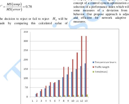
The applicability of our approach to adaptive network system behavior has been tested under different temperature levels and these measurements are used to display a performance graph (see figure 7). The concept of a control system optimization comprises a selection of a performance index which will minimize some measures of a deviation from the ideal behavior. Our propose approach is adjudged good and efficient for network adaptive behavioral measures.

Figure 7: Network Adaptive Behavior

5. CONCLUSION AND FUTURE WORK

Adaptive system implies that the system is capable of accommodating unpredictable environmental changes, whether these changes arise within the system or external to it. This concept has a great deal

(6)

reliability. In this paper, we designed frame work algorithms to carry out real – time traffic, capture the traffic through a sample run of these algorithms. The level of performance is measured by the mean value of temperatures using an ANOVA statistics and the measurements are used to display a performance graph. The concept of a control system optimization comprises a selection of a performance index which will minimize some measures of a deviation from ideal behavior. A fail to re ject H0 decision is

interpreted as the conclusion as there is no evidence of a difference due to the level of the tested factors. In other words, the temperature does not have a significant effect on the rate of network performance. In most control systems , small deviation in parameter values from their design values will not cause any problem in the normal operation of the system, provided these parameters are inside the loop. If system parameters vary widely according to environmental changes, the system may exhibit satisfactory response for one environmental condition but may fail to provide satisfactory performance under other conditions. Our propose approach is therefore adjudged an effective design for network adaptive behavioral measures. The solution to an optimal control problem may not exist if the system considered is not controllable and observable. Then it is necessary to know the condition under which a system is controllable and observable and this is a reference for future work.

REFERENCES

[BLV98] Yogesh Bhumralkar, Jeng Lung, Pravin Varaiya - Network Adaptive TCP slow Start, University of California, Berkeley, (1998).

[CZ10] W. Chen, Z. Zhang - Globally Stable Adaptive Back stepping Fuzzy Control for Output Feedback Systems with unknown High-Frequency Gain Sign, Fuzzy Sete and Systems, Vol. 161, No, 6, pp 821 – 836, (2010)

[Dob08] Simo n Dobson - An Adaptive System Perspective on Network Calculus, with Applications to Autonomic Control, International Journal of Autonomous and Adaptive Communications System,(IJAACS) Volume 1, Number 3, (2008)

[G+11] Joao V. Gomes, Pedro R. M. Inacio, Manela Pereira, Mario M. Freire, Paulo P. Monteiro - Identification of Peer – To – Peer VoIP Sessions Using

Entropy and Codec Properties. IEEE Transactions on Parallel and Distributed Systems, Volume x, No. x, (2011).

[Joh76] Robert R. Johnson - Elementary Statistics, Duxbury Press, North Scituate, Massachusette, Pages 449 – 470 (1976)

[LLS03] Leorunas Lymberopoulos, Emil Lupu, Morris Sloman - An Adaptive Policy Based Framework for Network Services Management, Journal of Network and Systems Management, Special Issues on Policy Based Management, 11:3, pages 277 – 303, (2003)

[MP13] Lepora N. Martinez, T. Prescott -

Active Touch for Robust Perception under Position Uncertainty, IEEE Proceedings of ICRA (2013).

[Oga86] Katsuhiko Ogata - Modern Control Engineering, Prentice Hall of India, Private limited, New Delhi, Pages 750 – 796 (1986)