Classification of Time Sequences
using Graphs of Temporal Constraints
Mathieu Guillame-Bert [email protected]
Artur Dubrawski [email protected]
Auton Lab, The Robotics Institute, School of Computer Science Carnegie Mellon University, Pittsburgh, United States
Editor:Luc De Raedt
Abstract
We introduce two algorithms that learn to classify Symbolic and Scalar Time Sequences (SSTS); an extension of multivariate time series. An SSTS is a set ofevents and a set of
scalars. Aneventis defined by a symbol and a time-stamp. Ascalaris defined by a symbol
and a function mapping a number for each possible time stamp of the data. The proposed algorithms rely on temporal patterns called Graph of Temporal Constraints (GTC). A GTC is a directed graph in which vertices express occurrences of specific events, and edges express temporal constraints between occurrences of pairs of events. Additionally, each vertex of a GTC can be augmented with numeric constraints on scalar values. We allow GTCs to be cyclic and/or disconnected. The first of the introduced algorithms extracts sets of co-dependent GTCs to be used in a voting mechanism. The second algorithm builds decision forest like representations where each node is a GTC. In both algorithms, extrac-tion of GTCs and model building are interleaved. Both algorithms are closely related to each other and they exhibit complementary properties including complexity, performance, and interpretability. The main novelties of this work reside in direct building of the model and efficient learning of GTC structures. We explain the proposed algorithms and eval-uate their performance against a diverse collection of 59 benchmark data sets. In these experiments, our algorithms come across as highly competitive and in most cases closely match or outperform state-of-the-art alternatives in terms of the computational speed while dominating in terms of the accuracy of classification of time sequences.
Keywords: classification, temporal data, sequential data, graphical constraint models,
decision forests, symbolic and scalar time sequences, supervised learning
1. Introduction
Learning to classify from labeled training data is one of the flagship capabilities of machine learning. Classification is commonly used to model flat-table data, and in applications involving more complex representations such as (time) sequences or graphs, the information is typically “featurized” or “flattened” to fit the flat-table representation paradigm, so that standard classification algorithms can be readily applicable. In the case of symbolic time-stamped sequences, popular featurization techniques include representing time-since-previous-occurrence of an event, or computing frequency of occurrence (or other statistics or measures) over moving windows of time. Perhaps, a preferable alternative is to instead use
c
classification algorithms capable of natively handling the temporal aspects of time-stamped sequences.
In this paper we introduce two parametric algorithms that belong to that specialized class. Both algorithms are designed to classify Symbolic and Scalar Time Sequences (SSTS); an expressive extension of the Time Series (TS) representation that remedies some of its lim-itations. In particular, SSTS extends the standard TS model by allowing non-uniform and asynchronous sampling, representing instantaneous sparse events as well as dense numeric sequences, and scaling well to highly-dimensional (multi-channel) application scenarios.
Both algorithms rely on a simple but expressive graphical pattern model for SSTS data called Graph of Temporal Constraints (GTC). A GTC is a conjunction of three types of conditions: (1) Existence of an event, (2) Constraint on the timestamp difference between two given events, and (3) Inequality constraints on the numerical values of a numerical time sequence at a time defined by a given event. Each GTC defines a Boolean function on an SSTS (or a TS).
The first algorithm presented in this paper, called the “GTC-Set”, bootstraps training SSTSs and extracts fitting GTCs to form an ensemble model. Unlike methods relying on extracting all possible patterns and then applying a feature selection, our first algorithm directly build a final set co-dependent discriminant GTCs (all extracted GTC are used and no feature selection is applied). For this reason, the set of build GTCs is much smaller than the set of all possible GTCs. At the end of the learning process, each thusly extracted GTC is used as an individual “voter” in the classification procedure.
The second algorithm, called “GTC-DF”, builds a bootstrapped decision forest where the condition in each decision node is defined as a GTC. Path of inference through each decision tree in this forest depends on whether a query STSS fulfills the constraints of the particular node’s GTC or not. Here again, the GTC attached to each node is directly constructed on-the-fly instead of being selected from a pool of existing GTCs.
To assess performance of the GTC-Set and the GTC-DF algorithms, we evaluated them on a diverse collection of 59 temporal sequence classification data sets (all of them are available publicly), and compared against 13 alternative algorithms found in the literature. Results show that our algorithms are highly competitive and in most cases outperform state-of-the-art considered alternatives, both in terms of computing speed and accuracy of classification. Our algorithms are especially competitive for unaligned temporal sequence data, i.e. the data for which the value of an observation at a particular time t has no distinct predictive value, or in other words: classification performance does not depend on when we start observing the data. We also show how the users can interpret learned models based on the proposed GTC representation. Interpretability is often an important factor that determines practical usability of machine learning solutions in the real world, and our presented framework satisfies this requirement well.
time
scalars eve
nts ee12 e3
s1
s2 s3
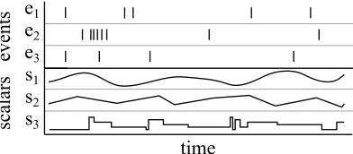
Figure 1: Example of an SSTS with three event symbols and three scalar variables.
2. Problem Definition
A Symbolic and Scalar Time Sequence (SSTS) is a temporal data set representation with a high power of expression. It is defined as follows:
Let E = {e1, . . . , en} be a set of n distinct symbols called event symbols. Let S = {s1, . . . , sm}be a set ofmdistinct symbols calledscalar symbols. Anevent is a tuplehei, xi
where x ∈ R is a timestamp. A scalar mapping is a tuple hsi, fii where fi is a function
R7→R;t→vthat maps each time-stamptto a valuev. Finally, asymbolic and scalar time
sequence d=hP, Qi is a tuple whereP is a set of events andQis a set of scalar mapping. By convention, an event of typeei is said to “happen” at timetifhei, ti ∈P, and the value
of the scalar sj at time t is fi(t) with hsi, fii ∈Q. Figure 1 shows an example of SSTS.
Note that an SSTS can contain several events with the same (event) symbol.
The SSTS classification problem is defined as follows: Given a set of labeled SSTSs and a set of unlabeled SSTSs drawn from the same underlying distribution, infer the labels of the unlabeled SSTSs.
3. Related Work
Published research into temporal data classification can be grouped into three categories:
distance based methods, flattening methods and model based methods. This categorization does not take into account possible data pre-processing steps.
Distance based methods rely on a definition of a distance between pairs of time series, and the use of a distance-based classification algorithm (such as e.g. k-nearest neighbors). If the distance metric requires tuning of its parameters to optimize the data fit, the observations available for training are split into separate training and validation samples. Methods falling into this category include nearest neighbor and Euclidean distance (NN+ED) (Ding et al., 2008), NN+L1 (Ding et al., 2008), NN+Linf (Ding et al., 2008), DTW (Berndt and Clifford, 1994), LCSS (Vlachos et al., 2002), ERP (Chen et al., 2005), EDR (Chen and Ng, 2004), DISSIM (Frentzos et al., 2007), SWALE (Morse and Patel, 2007), TQUEST (Aßfalg et al., 2006).
statistics of the temporal data computed over moving time windows (mean, standard de-viation, skewness, kurtosis, etc.), parameters prevalent in forecasting applications (trends, periodicity), and popular temporal signal projections (Fourier Transform, Wavelet Trans-forms, Singular Value Decomposition, etc.). Methods that rely on extracting a large amount of patterns from raw data followed by either applying feature selection and/or applying one of the classification algorithms to identify combinations of patterns that are effective on the task, fall into this category (Guillame-Bert and Dubrawski, 2014; Batal et al., 2012; Liu et al., 1998; Li et al., 2001). In this case, large amount of patterns are extracted according to user defined constraints (e.g. minimum support) and scores (e.g. F1), before being fed into a classifier. However, these methods are often slow because of the large amount of patterns to extract. And because discriminant power for classification does not always imply high score for a pattern, the methods may miss important patterns.
Finally, direct-model-based methods directly extract from data a model that contains temporal information. Examples of such methods include Rodr´ıguez and Alonso (2004) and Deng et al. (2013) who have modified the decision forest framework (Breiman, 2001) to handle time series. In these approaches, conditions in the non-leaf nodes of the decision trees are of the form fi(t1, t2)< α withfi(t1, t2) function computing a predefined statistic
on all time series points between t1 and t2. For Rodr´ıguez and Alonso (2004), fi(t1, t2) is
the mean, standard deviation or the dynamic time warping distance to a template time series. For Deng et al. (2013), f is either the mean, standard deviation, or an estimation of the slope. Methods presented in Rodriguez et al., Deng et al. and Ye and Keogh (2009) do not fit the flattening paradigm because the features or conditions are determined at the time when the model is built instead of at a separate pre-processing stage. Inductive Logic Programming (Muggleton, 1991) (ILP) is a general framework that is capable to express many temporal patterns. Rodriguez et al. (2000) has shown an example of how to use ILP to classify time series. However, from our experience and because of their general nature, it is unclear how ILP solvers could learn efficiently temporal patterns containing time constraints which are not predefined by the users. The two algorithms proposed in this paper fall in this last category of methods.
algorithm (i.e. the labels are used in the pattern extraction stage), and it does not contains a pattern selection nor training of a classifier stages: All extracted patterns are directly and independently used. Such simple application of extracted patterns is only possible because of the specific extraction of the GTC-Set algorithm. For example, directly and independently applying all patterns extracted from a frequent itemset mining algorithm would lead to poor results.
Supervised Descriptive Rule Discovery (Novak et al., 2009) (proposed as a unification of Contrast Set Mining (Bay and Pazzani, 2001), Emerging Pattern Mining (Dong and Li, 1999), and Subgroup Discovery (Kl¨osgen, 1996)) is the supervised extraction of association rules from labeled transactional data sets for the purpose of user interpretation and data discovery. Rules are extracted to maximize a user defined interest score often measuring a lift-life measure or a statistical distance from a null-space model. Unlike pattern-based classification, these rules are not designed to be used for classification. In section 7.7, we discuss how to extract a small but representative subset of GTC patterns from set of patterns extracted by the GTC-Set algorithm. While being less performant for the classification task than the original set of patterns, the selected set of patterns aims to be easier to interpret by a user. The GTC-Set algorithm conjugated with pattern selection method can be seen as a solution to Supervised Descriptive Rule Discovery on SSTS. Interestingly, and contrary to most of the Supervised Descriptive Rule Discovery literature, the proposed method build an interpretable model from a classifier.
Unlike itemset mining, sequential mining allows for the definition and use of a relation of order in between items. This order is often used to represent the temporal sequence of the items: One item can be anterior, posterior or concurrent to another item. However, time distance is not taken into account by sequential mining, and in many dynamical systems, relations such as the time distance or the overlapping between items is discriminant.
In the literature, learning algorithms dealing with temporally discrete data (e.g. time point events) face the challenge of representing and extracting temporal constraints between pairs of time points. In most of the literature such constraints are represented with a subset
C of R: Given two data points with timestamps respectively t1 and t2, the constraint is satisfied if and only if t2−t1∈C.
This formulation has a high power of expression, but it can be prone to over-fitting given the potentially infinite number of candidate patterns and many available and applicable algorithms for pattern extraction are intractable. Solutions found in the literature rely on two principles: Constraining possible values of C, and/or defining an inexpensive to optimize score function on C. The simplest and the most popular solution is to require for the user to specify a small set of candidates for C (Mannila et al., 1997). Rodr´ıguez and Alonso (2004) and Rodriguez et al. (2000) only consider segments of the form [2i,2j] where
defined by the user {[ai+b, a(i+ 1) +b]}i∈[m,n]. Recursively, the algorithm selects the set of segments that maximizes information gain. The maximization problem is solved approximately using a forward or backward gradient descent optimization. The resulting constraint is not necessarily a contiguous segment. Guillame-Bert and Dubrawski (2014) consider all combinations [bi, bj] where{bi}are provided by the user, andiandjare selected
to maximize information gain. All possible combinations ofiandjcan be evaluated thanks to an efficient specialized data encoding.
The algorithms proposed in this work rely on learning constraints of the type [a, b] (aand
b are not constrained). aand b are selected to maximize information gain. This is a strict improvement over Guillame-Bert and Dubrawski (2014). Efficient and exact, according to the information gain criterion, extraction ofaandb is one of the main results of this work.
4. Graphs of Temporal Constraints
A Graph of Temporal Constraints (GTC) is a set of temporal constraints represented as a graph.
Definition 1 A GTC is defined by a set of testsQ={q1, . . . , qn}and a set of constraints
C={c1, . . . , cm}.
A test qi is defined by an event symbol, a positive or negative flag, and a (possibly
empty) set of scalar tests. A qi test with a positive flag is true at time t if an event with
the given event symbol exists at time t, and if all its scalar tests are true at time t. A test with a negative flag is true if and only if the same test with a positive flag is impossible to satisfy.
A scalar test is an inequality constraint based on a scalar mapping value at a time t defined by the node. In this work, scalar tests are restricted to be inequalities between a single scalar mapping term and a threshold value.
A constraint ck is defined by two tests qi andqj, a positive or negative flag, and R⊂R
(a subset of the real numbers). A constraint with a positive flag is true if its both tests are true respectively at timeti andtj and iftj−ti ∈R. A constraint with a negative flag is true
if and only if the same constraint with a positive flag is false. In other words, a negative constraint [a, b]is equivalent to the disjunctive constraint ]−inf, a[∪]b,+ inf[. Additionally, we restrict GTC not to have conditions/edges starting from a negative test/node.
This restriction is similar to the apriori constraint for association rule mining, and it guaranties that if built iteratively, the GTCs at successive steps have decreasing support.
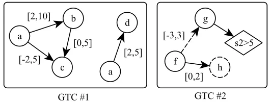
A GTC can be seen as a directed graph were each vertex expresses the existential condition for an event (conditioned by a symbol), i.e. a test, and where each edge expresses a temporal constraint between the vertices it connects, i.e. a constraint. A GTC can contain undirected cycles and disconnected components. Fig. 2 shows two examples of GTCs.
Let us now introduce some aspects of notation used for describing GTCs. A GTC instance {ki}i∈1,...,n assigns times ki to each of the tests qi of GTC A so that all tests and
all constraints of A are true. By convention, A(d) denotes the set of instances of A in an SSTSd. Note that different instances can partially overlap with each other. By convention,
A is true in an SSTS d if d contains at least one instance of A, i.e. |A(d)| > 0. Trace
GTC #1 a
b
c
d
a [2,10]
[-2,5]
[0,5]
[2,5]
GTC #2 f
g
h s2>5 [-3,3]
[0,2]
Figure 2: Two examples of GTCs. Dashed vertex (or edge) represents a vertex (or edge) with a negative flag. Diamond shapes represent scalar tests.
with the test qi for any instances of A on d: T(qi, d) ={ki | ∀{k1, . . . , ki, . . . , kn} ∈A(d)}.
Given a set of SSTS D = {d1, . . . , dn}, A(D) is the subset of SSTS for which A is true:
A(D) ={di|di ∈D with|A(di)|>0}. By convention, a GTC without tests is always true.
Finally, given a set of SSTS D, the support of A is the fraction of SSTS where A is true:
supp(A) =|A(D)|/|D|.
Testing the existence of a GTC in an SSTS (i.e. computing the existence of instances) can be done by (1) Extracting a set of spanning trees of the GTC (one tree for each of the GTCs disconnected components), (2) Independently matching each tree to the SSTS records while continuously, and (3) Checking any additional constraints that were not the part of the spanning trees. The cost of testing a GTC is polynomial with the number of events and exponential with the number of nodes. The smaller the surfaces of the temporal constraints between nodes, the less extensive the exploration, and the faster the GTC matching. However, in practice (cf. Experimental evaluation section below), the cost of testing GTCs is insignificant in comparison to the cost of learning these GTCs. It appears that because the constraints on the edges are selected to be discriminant, they tend to be restrictive and help in pruning large parts of the exploration space.
To the best of our knowledge, GTC is a novel representation, but it can be related to some existing temporal pattern representation frameworks. The closest are the Temporal Constraint Network (TCN) of Dechter (1991), the Chronicles of Dousson and Vu Duong (1999) and the Tita rules of Guillame-Bert (2012). TCN and Chronicles can be seen as reduced cases of GTCs in which tests and constraints do not have negative flags and in which there are no scalar tests. Tita rules allow node negation but do not allow undirected cycles or disjoint components.
5. Classification with GTCs
In this section, we introduce two SSTS classification models that use GTCs as their building blocks. The first model we call GTC-Set. A GTC-Set is an unstructured set of labeled (assigned to represent a particular unique class of STSS) GTCs. Given an unlabeled SSTS
a b c
c1
a b c
c2
a d
a b c c
c2
a a a
c3
b b c1
c1
(a)
a
a b
a d a b
c
c1 c2
parentgrand-parentgrand-parent
parent positive node
negative node
c3
c1 c3
(b)
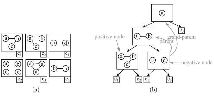
Figure 3: Examples of a GTC-Set (a) and a tree in a GTC-DF (b). Class labels in the leaf nodes are denoted withci.
The second model we call GTC Decision Forest (GTC-DF). A GTC-DF is a set of
decision trees where each non-leaf node is associated with a particular GTC and it has two children. Additionally, the GTC attached to a decision tree node is constrained to be directly derived from the GTC of the parent node if connected by a positive decision tree branch, and from the grandparent node otherwise. This constraint is important and it will be discussed and justified in the next section. When applying a GTC-DF to classify a query in the form of a STSS, the decision trees are independently traversed in a familiar way. Upon arrival in a node, its associated GTC is tested for fitness to the data and the result of this test determines the direction of further traversal. As in the original decision forest algorithm (Breiman, 2001), class label distributions are agglomerated across the final active leaf nodes of each component tree, in order to obtain the joint prediction. Figure 3 shows an example of a tree in a GTC-DF.
Independence of components in GTC-Sets makes these models somewhat easier to in-terpret by the users than GTC Decision Forests because each of them can be considered individually. Conversely, interpretation of a GTC Decision Forest model, as well as its infer-ence process in response to a particular query, requires consideration of GTCs corresponding to the subsequent nodes in each tree.
6. Learning Temporal Patterns
Both algorithms build GTCs by recursively applying constructive operations. In the process, selection of the next operation to apply is guided by maximizing the local informa-tion gain. This secinforma-tion presents GTC building operainforma-tions, defines the concept of informainforma-tion gain of an operation, presents how to efficiently identify the operation with the highest in-formation gain, and details the main loops of the two algorithms. Our proposed solution to how to efficiently extract optimal temporal constraints for the edges in GTCs is one of the main novelties of this work.
6.1 Constructive Operations on GTCs
Constructive operations on a GTC include:
O1: Addition of a new test (i.e. addition of a vertex),
O2: Addition of a constraint between two existing tests (i.e. addition of an edge), O3: Addition of a scalar test to an existing test,
O4: Addition of a new test and addition of a constraint between this test and an already existing test.
Each operation requires specific parameters. O1 requires an event symbol and a posi-tive/negative flag. O2 requires two existing tests, a flag and a subset of R. O3 requires an existing test and a scalar test defined by a scalar symbol, a threshold value and an inequal-ity direction (< or≥). O4 requires a combination of arguments of O1 and O2. Note that, because of the threshold value of the scalar test in O3, and because the need for a subset of Rin O2 and O4, these operations have an infinite number of possible parameter values. Operation O4 is equivalent to operations 1 and 2 combined. We justify its existence later.
Both proposed algorithms require for the set of positive SSTS according to a GTC to be monotone decreasing when applying operations: Given a set D of SSTSs, a GTC A, an operation O and B the result of O on A. Algorithms require for the set of positive SSTSs according to B to be contained in the set of positive SSTSs according to A i.e.
B(D)⊂A(D). This implies that each operation reduces (albeit not strictly) the support of the GTC it is applied to. For this reason, operations O2-O4 cannot be applied on negative nodes.
The result of the negation of an operation O on a GTC A is a GTC B0 such that
∀d∈ D, A(d) ⇒ (B(d) ⇔ ¬B0(d)) and ¬A(d) ⇒ (¬B(d)∧ ¬B0(d)), where B is the result of O on A. Note: ⇔ and ¬ are respectively the logical equivalence and logical negation. Except for trivial cases, the GTC resulting from the negation of an operation is more complex than the result of the operation. In the case of fully connected GTCs, the size of the GTC resulting from the negative operation is twice the size of the result from the direct operation. Instead, we define the approximate result of the negation of an operation. This approximation is not exact but it provides reasonable results as presented in Section 7.
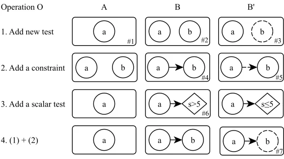
Whether to use or not the approximate negation is the main difference between the two proposed algorithms. Figure 4 illustrates these operations and their associated approximate negations. Adding a constraint to a test with a negative flag would violate the support reduction property and it is therefore forbidden. The goal of O4 is to allow creating a connected test with a negative flag without violating the support reduction requirement.
a a b
a b a b a b
a a s>5 a s≤5
a a b a b
a b
1. Add new test
2. Add a constraint
3. Add a scalar test
4. (1) + (2)
B B'
A Operation O
#1 #2 #3
#4 #5
#6
#7
Figure 4: Illustration of the constructive operations on GTCs. Each row of graphs rep-resents a specific operation. Column A reprep-resents the initial GTC. Column B shows the result of executing the particular operation on the initial GTC. Col-umn B’ depicts the result of the approximate negation of the operation. Dashed nodes and edges represent respectively tests and constraints with negative flags. Diamonds represent scalar tests. Description of the GTCs: #1: An event of type
ais present. #2: An event of typeaand an event of typeb are present. #3: An event of typeais present, but no event of typebis present. #4: An event of type
aand an event of typeb are present, and they satisfy the constraint of the edge. #5: An event of typea and an event of typeb are present, and they satisfy the complementary constraint of the edge. #6: An event of typeais present at time
tsuch that the scalarsvalue is greater than 5 at time t. #7: An event of typea
is present at time ta such that there is no event b at time tb such that ta and tb
satisfy the constraint.
approximate result of the negation of this operation. A expresses that “There is an eventa
followed by an eventbbetween 0 and 2 time units”. B expresses that “There is an eventa
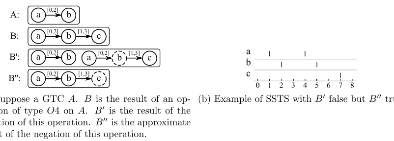
followed by an event bbetween 0 and 2 time units, itself followed by an event cbetween 1 and 3 time units”. B0 expresses that “There is an eventafollowed by an eventbbetween 0 and 2 time units, but there is not an event afollowed by an eventb between 0 and 2 time units, itself followed by an eventc between 1 and 3 time units”. B00 expresses that “There is an event a followed by an event b between 0 and 2 time units, itself not followed by an eventc between 1 and 3 time units”. Figure 5b shows an SSTSB00 is true but whereB0 is not.
6.2 Information Gain Maximization
a b A:
a b
B:
a b
B':
a b
B'':
c
a b c
c
[0,2]
[1,3] [0,2]
[0,2]
[0,2]
[0,2] [1,3]
[1,3]
(a) Suppose a GTC A. B is the result of an op-eration of type O4 on A. B0 is the result of the negation of this operation. B00 is the approximate result of the negation of this operation.
a b c
0 1 2 3 4 5 6 7 8
(b) Example of SSTS withB0 false butB00 true.
Figure 5: Illustration of the negation and the approximate negation of an operation.
distribution of their labels
H(D) =X
i
−pi(D) logpi(D)
, with pi(D) representing the relative frequency of label i in D. Additionally, we assert
0 log 0 = 0.
Given a set of SSTSs D = d1, . . . , dn, a GTC A such that A is true for all di, and an
operationO, ifB is the result of O on A, then information gain IG of the operationO on
A can be defined as
IG=H(D)−|B(D)|
|D| H(B(D))−
|D\B(D)|
|D| H(D\B(D))
, whereH(D) is commonly called the initial (prior) entropy, and the rest of the right hand side of the formula is the weighed final (posterior) entropy.
During the training stage, given a GTC A, both algorithms rely on finding such con-structive operation and its parameters that maximize the information gain. Except for operation O1, testing and evaluating the information gain over the range of possible param-eter values is in most cases infeasible because of the infinite number of tests it might involve. We propose a solution based on the following four considerations: (1) Instead of considering all subsets of R (operations O2 and O3), we only consider contiguous segments of R; (2) Since each finite data set consists of a finite number of SSTSs, and each SSTS is composed of a finite number of events, there is only a finite number of parameter values that need to be considered; (3) The procedure of extracting a plausible threshold for an operation O3, and the corresponding segments of R, can be optimized for computational speed with an appropriate algorithm and an appropriate internal data structure; and (4) Random sam-pling can be used as an option to further speed up the extraction of the optimum threshold and the optimum segments of R.
6.3 Learning Decision Trees and Forests of GTCs
We build decision trees and forests of GTCs similarly to how standard decision trees and forests are built (Quinlan, 1993; Breiman, 2001). The two differences are that: (1) Each decision node of a GTC tree is assigned a GTC instead of a single threshold condition on a single data feature as it is the case of the standard model; and (2) The structure of a GTC representing a node of a GTC tree is heavily constrained by the structure of the GTCs of its parent and grand-parent nodes.
The algorithm for training a GTC tree starts with a single empty GTC and it looks for the operation on it that yields the highest information gain. This operation is then applied, and the resulting GTC is used to define the root node constraint. The root node constraint is used to split the training SSTSs into two complementary subsets. The same procedure is further recursively applied to these subsets and additional nodes are appended to the tree until a stopping criterion is met. The GTC of a positive node of the decision tree will be derived by applying a single operation on the GTC attached to its parent. The GTC of a negative node of the decision tree will be derived by applying a single operation on the GTC attached to its grand-parent. This restriction has three benefits: (1) Search space for the new GTC is limited and therefore fast to explore. (2) The new GTC is constrained and therefore the risk for it to over-fit is mitigated. (3) GTCs of an arbitrary complexity can still be derived. A GTC Decision Forest (GTC-DF) can be obtained by bootstrapping data for GTC decision tree learning from the training set of SSTSs. Note that we typically also bootstrap the GTC-Set models and in fact use ensembles of GTC-Sets, cf. Algorithm 2. Pseudocode in Algorithm 1 provides details.
Algorithm 1:Extraction of a GTC decision forest from data.
input : D: A set of SSTSs
b: The number of bootstrap iterations (e.g. 20)
l: The minimum number of times a GTC is used (e.g. 5)
output: M: The set of extracted labeled GTCs
Algorithm
fori ←1 to bdo
A←an empty GTC
recursive build(D, A)
Subroutinerecursive build(D,reference to A)
M ←M∪A
if |A(D)|< l then
label(A)←most frequent class inD withAtrue return
o←find the operation onAwith the highest information gain
B2←A
A←result ofO onA B1←A
setB1 andB2 to be respectively the positive and negative children ofA
recursive build(B1(D), B1)
6.4 Learning Sets of GTCs
This sub-section introduces the algorithm to extract a GTC set from data. This algorithm starts with a single empty GTC A and looks for the operation with the maximum infor-mation gain to extend its structure. This operation and the approximate negation of it are applied to the GTCAto create two new GTCs, respectivelyB1andB2. Ais then removed.
The same process is next recursively applied to bothB1 and B2 until a stopping criterion is met. Finally, each remaining (i.e. non removed) GTC is assigned to the most common class of the SSTS where it is true. Note that because of the approximated negation B1(D)
and B2(D) are not necessary disjoint (the last line of the Algorithm 2).
Algorithm 2:Extraction of a GTC set.
input : D: A set of SSTSs
b: The number of bootstrap iterations to execute (e.g. 20)
l: The minimum number of times a GTC is used (e.g. 5)
output: M: The set of extracted labeled GTCs
Algorithm
A←an empty GTC
fori ←1 to bdo
M ←M ∪recursive build(D, A)
Subroutinerecursive build(D,A)
if |D(A)|< l then
label(A)←most frequent class inD withAtrue returnA
o1←find the operation onAwith the highest information gain
o2←approximate negation ofo1
B1←result ofo1onA
B2←result ofo2onA
returnrecursive build(B1(D), B1)∪recursive build(B2(D), B2)// Note that it
is not required nor expected that B1(D)∩B2(D) =∅
6.5 Finding the Optimal Scalar Tests
A scalar test is defined by an existing test qi, a scalar symbol sj, a threshold value α and
the direction of inequality (< or ≥). The problem of finding the optimal threshold value is different but related to the problem of finding the optimal threshold in the decision tree learning algorithm C4.5 (Quinlan, 1993). Unlike C4.5, our algorithms need to consider several scalar values for each observation/SSTS: one scalar value for each GTC instance on a given SSTS.
To identify the optimal scalar test, the algorithm considers all possible existing tests
qi with a positive flag, every scalar symbol sj, and both inequality directions < and ≥.
For each of these values, the algorithm computes the optimal threshold value α as follows. Consider a GTCA, the set of training SSTSD={di}1..n, the scalar symbolsj, the existing
as follows:
L[j,1] =
min({sj(x)|∀i, x∈T(qj, di)}) if the inequality is <
max({sj(x)|∀i, x∈T(qj, di)}) if the inequality is ≥
L[j,2] =label(dj)
where T(qj, di) is the trace of the testqj on the SSTS di (see the definition in Section 4).
Next, this matrix is sorted according to its first column and all possible threshold values are evaluated in a sequence. α is defined as the threshold with the highest information gain. Algorithm 3 shows the details of these operations:
Algorithm 3:Finding the optimal threshold valueα for a new scalar test.
input : L: An×2 matrix as described in section 6.5.
output: α: the optimal threshold
SortLaccording to the first column values
h0←+∞;i0 ←0 ;w←f alse
X ← {0} ×C withCthe number of classes
Y ←such that Yi is the number of SSTS of classci
fori←1 ton−1 do
XL[i,2] ←XL[i,2]+ 1
YL[i,2]←YL[i,2]−1
if L[i+ 1,1]6=L[i,1]∧(L[i+ 1,2]6=L[i,2]∨w)then
w←f alse
h←entropy(X)i+entropy(Y)(n−i) if h < h0 then
h0 ←h; i0←i
else
w←true
α←(L[i0,1] +L[i0+ 1,1])/2
6.6 Finding the Optimal Segment of R
Operations O2 and O4 require specification of a time constraint. In this work, we restrict time constraints to be contiguous segments [a, b]∈R, albeit in general this restriction can be lifted without harm. The data set being finite, the number of meaningful candidate boundaries foraand b is also finite.
Given a GTC A and an operation O2 or O4 to apply, we define M(dk)⊂R as follows. For operation O2, given two tests qi and qj of A,M is defined as M(dk) ={x1−x2|∀x1 ∈ T(qi, dk), x2 ∈ T(qj, dk)}. For operation O4, given an existing test qi of A and an event
symbolej,M is defined asM(dk) ={x1−x2|∀x∈T(qi, dk),∃hej, x2i ∈dk}. Note thatM
is computed from the trace T that is itself computed during the GTC evaluation.
By design, (1) If A is not valid on an SSTS dk, then M(dk) is empty; and (2) If A is
valid on an SSTS dk, then the GTC resulting from applying the current operation with
constraint [a, b] on A is valid on dk if and only if ∃x∈M(dk) such thatx∈[a, b].
We defineY =S
kM(dk), and Yi to be the ith smallest element ofY. Finally, we define
{Y1} ∪ {Y|Y|}. In case of large data sets, or in case of small data sets with high risk of over-fitting, the set of candidate Z can be randomly sampled down. Such down sampling is in essence equivalent to attribute sampling used e.g. in Random Forest. In practice, this significantly speeds up the search for the optimal time constraint without reducing the model accuracy because of the redundant nature of the decision tree or decision set models. We observed experimentally that limiting Z to 40 elements (i.e. 402 interval candidates) does not impact the models’ empirical accuracy.
Finding the segment [a, b] that maximizes the information gain is an optimization prob-lem in a finite and countable two dimensional space. The naive and direct solution to this problem requires evaluating a GTC on each SSTS for each unique point in the search space (i.e. for each possible (a, b) ∈ Z2 with a < b). This solution leads to the worst case com-putational cost ofO(|Z|2nE) withnbeing the number of SSTSs and E the computational
cost to compute the instances of a GTC on an SSTS. This cost may easily become pro-hibitively expensive for any realistically complex application. An alternative, more efficient solution is to iterate overM to evaluate application of the GTC. This solution only requires evaluating the initial GTC once, it does not require evaluating the resulting GTC, and it has a computational cost of O(|Z|2n+En). It allows us to handle much larger problems
than when using the naive approach.
Instead of these two implementations, we propose a third solution with a time complexity of O(|Z|2+nE) (instead of O(|Z|2nE) of O(|Z|2n+En), as above). This new approach
relies on the two following properties: (1) If h ∈M(dk), then the GTC resulting from the
current operation with the time constraint [h, h] is true on the SSTS dk; (2) If the GTC
with the new constraint [a, b] is true on the SSTSdk, then all GTCs with a time constraint
[a0, b0]⊃[a, b] will also be true on the SSTSdk.
The last solution relies on building a |Z| × |Z| ×(C −1) matrix P where C is the number of classes in the classification problem. After being built, each element ofP[x, y, z] represents the number of SSTSs in training data which belong to classzand that match the GTCAafter it was subjected to the new operation with the time constraint [Zx, Zy]. Once
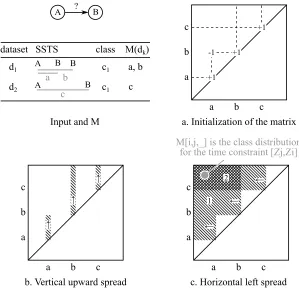
the matrix P is computed, search for the optimal time constraint can be done in one pass overP by iterating overx and y, then overz in the inner loop. Algorithm 4 shows how to efficiently construct matrixP. Note that in practice, search for the optimal time constraint can be merged with the last “for” loop of the algorithm. Figure 6 illustrates the Algorithm 4 step by step using a small example. Also note that while we useP to optimize information gain,P can be used to optimize any metric that relies on GTC matching counts.
7. Experimental Evaluation
In this section we report and discuss performance of the two proposed algorithms (GTC-DF and GTC-Set) as compared to a wide variety of alternative approaches found in literature. The algorithms are evaluated on a collection of 59 unique data sets described below. All these data sets are publicly available online.
7.1 Synthetic Data (1 set)
Algorithm 4:Building matrixP.
input : Z: The set of candidate boundaries.
M: The “meet” sets.
output: P: MatrixP.
// a. Initialization
P ←a |Z| × |Z| ×(C−1) matrix filled with zeros
fork= 1to |D|do
k← −1;c←class ofdk
if c=Cthen continue
m←M(dk)// mi is the ith smallest element of m.
fori= 1to |m|do
j←such thatZj ≤mi < Zj+1 // Note: i7→j is monotonically increasing
P[j, j, c]←P[j, j, c] + 1
if k6=−1 then P[j, k, c]←P[i, k, c]−1
k←i
// b. Vertical upward spread
fori= 1to |Z|do
X← {0} ×(C−1)
forj =i to |Z|do
X←X+P[j, i, ]
P[j, i, ]←X
// c. Horizontal left spread
fori= 1to |Z|do
X← {0} ×(C−1)
forj =i to 1do
X←X+P[i, j, ]
// Note: Here X contains the class distribution for the candidate GTC with time constraints [Zj, Zi].
P[i, j, ]←X
events from the set A, B and C, respectively at times ta, tb and tc. For each SSTS, ta is
sampled uniformly from [0,200], andtb andtcare sampled uniformly from [ta−15, ta+ 15].
If |ta−tb|<10 and |ta−tc|<10 and |tb−tc|<10, then the SSTS is labeled as class 1.
Else, if |ta−tb|<10, then the SSTS is labeled as class 2. If none of these conditions are
valid, the SSTS is labeled as class 3. This data set aims to evaluate our algorithm capability of correctly learning temporal constraints from data. The synthetic data set as well as a Python script used to generate it are available atmathieu.guillame-bert.com/dataset.
7.2 UCR Time Series Classification Repository (41 UCR Data Sets)
b c a
+1 -1 +1
+1
a b c
a. Initialization of the matrix c1
c1
a, b
c
c
a b
b c
a a b c
b. Vertical upward spread
→
→
→
c. Horizontal left spread
b c
a a b c
→ →
→
1 2
M[i,j,_] is the class distribution for the time constraint [Zj,Zi] dataset SSTS class M(dk)
d1
d2
A ? B
A B B
A B
Input and M
Figure 6: Step by step illustration of Algorithm 4 to constructM, matrixP, and the optimal time interval constraint.
Dynamic Time Warping (DTW) restricted to a very small shift coupled with one nearest neighbor) and algorithms designed for “flat” data sets (such as e.g. SVM) can be very com-petitive. The UCR data sets are organized into two groups: Group 1 (18 sets) and Group 2 (23 sets). The number of classes, number of time series, and their lengths, vary in these data sets respectively from-to [2,50], [56,7164] and [60,637] for Group 1, and [2,25], [322,9236] and [28,1882] for Group 2. It appears that the sets in Group 2 are on average larger than sets of Group 1. These data are available athttp://www.cs.ucr.edu/∼eamonn/time series data.
7.3 16 Rotated UCR Data Sets
The original data
A rotated copy
Class 1 Class 2 Single observations (Class 1)
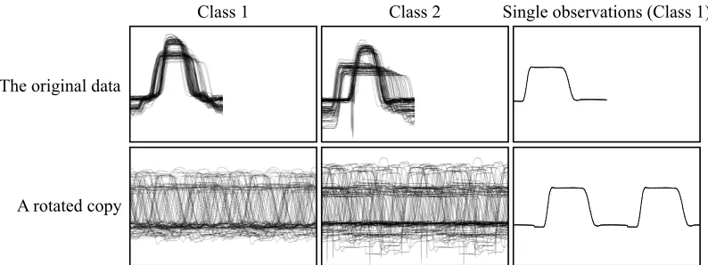
Figure 7: The original and one rotated copy of the UCR Gun Point data set.
well-defined initial setting. We call this modified collection of benchmark data the “Rotated UCR data sets”.
The rotation is performed as follows: We break any potentially pre-existing alignment of a data set by randomly and independently shifting each time series in it versus others. Given a time seriesX= [x1, . . . , xn], the rotated copy is defined asX0 = [xi, . . . , xn, x1, . . . , xn, x1, . . . , xi−1] withibeing a uniformly random integer drawn from the range [1, n] and
unique to each time series. In order to avoid disturbing local patterns (if they exist), the rotated series are doubled in length with regard to the originals. To enable comprehensive evaluation, we independently generate 10 rotated copies for each of the originals and use each of these copies independently in experiments. The reported classification performance will be computed by averaging the results obtained from the 10 rotated copies. To avoid excessive computation costs, we chose to rotate all but two UCR Group 1 sets. As an example, Figure 7 shows the original UCR Gun Point data and one of its rotated copies.
7.4 Internal Bleeding Detection Data Set (1 Set)
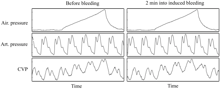
Undetected internal bleeding during and after surgical procedures is a major medical con-cern. Early and reliable detection of internal bleeding is therefore considered a significant medical research problem. We assembled the Bleeding Detection Data Set from vital signs measured at high frequency (250Hz) using a bed-side hemodynamic monitoring system. The collected measurements include arterial blood pressure, central venous pressure, and airway pressure. The data has been collected from a cohort of 52 healthy pigs subjected to induced slow bleeding. Each animal has been sedated, instrumented, left to rest for half an hour, and then bled at the fixed rate of 20mL/min. From the vital sign records of each pig, we randomly sampled two 30 second long segments of data: One from the resting period before and one approximately 2 minutes into the bleeding. Pre- and post-bleeding segments are respectively labeled as negative and positive. Unlike in the UCR data sets, the SSTSs (vital signs) are not temporally aligned: The starting point of observation is effectively arbitrary. Moreover, the data is multivariate.
Air. pressure
Art. pressure
CVP
Time Time
Before bleeding 2 min into induced bleeding
Figure 8: Four second samples of vital sign time series collected from one pig in pre-bleed phase (left) and 2 minutes into the induced bleeding (right). Note that in practice, vital signs of different animals tend to look less similar than vital signs of a same animal before and after bleeding. Air. pressure stands for Airway pressure. Art. pressure stands for arterial blood pressure, and CVP stands for central venous pressure.
that limit by considering SSTSs observed at a 2 minute mark into bleeding, when the data is not yet visually differentiable to expert clinicians. Figure 8 shows small parts of the pre-bleed and 2-minutes-in snapshots of vital signs data observed for one animal. The internal bleeding detection data set is available atmathieu.guillame-bert.com [Guillame-Bert].
7.5 Experimental Setup
Purposive featurization of time sequence data can sometimes significantly impact perfor-mance of the resulting models. In order to avoid obfuscating the relative perforperfor-mance of various algorithms being compared in this paper, we decided to not invest time and effort to produce advanced and potentially informative algorithm-specific featurizations of raw data. Instead, we relied on two basic statistics (moving averages and moving standard deviations), and we marked easily detectable peaks manifesting in the scalar data using a simple threshold criterion on the signal’s second order derivative.
All considered algorithms have been implemented (or re-implemented) in C++ to ensure fairness of comparison. The computation times reported include training and evaluation over the complete 10-fold cross-validation cycles. This allows fair comparisons of lazy (e.g. 10NN) and non-lazy (e.g. our methods) algorithms. Experiments have been performed on a 3.4GHz i7 8-core processor with 16GB of main memory. Multiple algorithms were slow when applied on the UCR data setStarLightCurves (StarLC). Algorithms taking more than one day of computation for the 10-fold cross-validation were stopped and the expected total computation cost was estimated from the completed iterations. For this reason, results on
7.6 Results
We compare our two algorithms against 13 related and relevant alternative classification algorithms for time series. The reference list includes: ED+NN: Euclidean Distance (i.e.L2
distance) with Single Nearest Neighbor (Ding et al., 2008), ED+kNN: Euclidean Distance withkNearest Neighbors (kis specified by the user),ED+CVkNN: Euclidean Distance with
kNearest Neighbors (kis determined through an internal loop 10-fold cross-validation exe-cuted on each training fold of the main 10-fold cross-validation loop),DTW+NN: Dynamic Time Warping (Berndt and Clifford, 1994) with Single Nearest Neighbor,DTWC+NN: Dy-namic Time Warping with Constrained Warping Window (Berndt and Clifford, 1994) with Single Nearest Neighbor,EDR+NN: Edit Distance on Real Sequence (Chen and Ng, 2004) with Single Nearest Neighbor, ERP+NN: Edit Distance with Real Penalty (Chen et al., 2005) with Single Nearest Neighbor, LCSS+NN: Longest Common Subsequence (Vlachos et al., 2002) with Single Nearest Neighbor, LCSSC+NN: Longest Common Subsequence with Constrained Warping Window (Vlachos et al., 2002) with Single Nearest Neighbor,
L-1+NN: L1 distance with Single Nearest Neighbor, L-inf+NN: L∞ distance with Single Nearest Neighbor, RF: Random Decision Forest (Breiman, 2001), SVM: Support Vector Machine Meyer et al., 2003,Default: Always return the most frequent class.
Algorithm parameters have not been tuned and were assigned to their meaningful default settings (except for k in ED+kNNCV), as follows. RF: maxNumTrees(30), minNumOb-servations(5), maxDepth(10). LCSS+NN: e(0.05 standard deviation). EDR+NN: e(0.25 standard deviation). LCSSC+NN: The maximum window is set to 25% of the data set length. It is worth noting that one could argue that the maximum window setting (c) of 25% is too high to operate DTWC and LCSSC on the UCR data sets, but we have chosen that for the three following reasons. Firstly, we have not tuned any algorithm parameters for specific data sets except for k in ED+kNNCV. Secondly, we have evaluated Euclidean Distance method being equivalent to DTWC with c=0%, and DTW being equivalent to DTWC with c=100%. Thirdly, c is a constraint parameter that only and strictly expands search space of the closest element when increased. We have experimented with alterna-tive settings of this parameter and we have indeed obtained slight variations of empirical accuracy of DTWC, but these variations have not materially changed performance rank-ings reported below. We therefore chose to evaluate DTWC+NN (and other constrained dynamic programming distances) with c=25% for consistency. It is significant to remark that we evaluated the original implementation of DTW (Berndt and Clifford, 1994). Sev-eral pruning criteria have been studied to reduce the computation time without impacting the classification performances, including the work of Keogh and Ratanamahatana (2005).
DTWC+NN: The maximum window is set to 25% of the data set length. ED+CVkNN:kis searched between 1 and 10. It is likely that optimizing parameters of each algorithm using internal cross-validation might improve their results, but it would significantly increase the computation time.
complete record for each animal is either entirely used for training or for testing in each cross-validation iteration.
Reported evaluation figures for the UCR data sets are not directly comparable with figures reported by Ding et al. (2008) or the figures available on the UCR Time Series web page: In Ding et al. (2008), evaluation results are computed with a “reversed cross-validation” where each of the n folds is successively used for training while the remaining
n−1 folds are used for testing. On the UCR Time Series web page, evaluation is performed with a train and test protocol.
Tables 1 and 3 respectively compile the observed classification errors of all algorithms on the UCR data sets and rotated UCR data sets. The average rank and median rank are also reported for each algorithm. Table 2 shows the cumulative computation times of training and testing cycles for each algorithm. Table 4 shows the accuracy, classification error, AUC scores and computation times of each algorithm when applied to the Bleeding Detection Data Set. Figure 9 shows the ROC of the GTC-DF and Random Forest models obtained for this data set.
First, both our algorithms show a 100% accuracy on the synthetic data. This simple experiment validates their ability to identify explicit temporal sequence patterns when they exist.
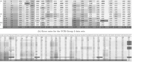
The experiments on the UCR data, rotated UCR data, and Bleeding Detection Data Set (Tables 1, 3 and 4), show consistently high performance of our algorithms in comparison to state-of-the-art alternatives. On the original UCR data, and when considering 13 other methods, GTC-DF and GTC-Set have the highest average and median ranks of accuracy (respectively a median rank of 2 and 2.5 for Group 1, and 2.5 and 2.5 for Group 2). The next best methods are ERP+NN (med. rank of 4.8) and DTW+NN (med. rank of 6) for Group 1, and SVM (med.rank of 4.5) and ERP+NN (med. rank of 5) for Group 2. It is worth noting that since the original UCR data sets are internally aligned, methods that rely on basic distance metrics (e.g. Euclidean Distance or DTWC with very strong constraints e.g.c=0.5%) tend to perform relatively well and are also cheap to compute.
measured on the individual data sets. The algorithms are sorted according to their average rank, and the two proposed methods top the sorted list.
(a) Error rates for the UCR Group 1 data sets.
Algo. avg.rank med.rank 50words Adiac Beef CBF Coffee ECG200 FaceAll Face4 GunPoint Lighting2 Lighting7 OSULeaf Trace 2Patterns Fish Synthetic Wafer Yoga
GTC DF 3.5 2 .225 .237 .300 .005 .036 .115 .045 .018 .015 .223 .196 .242 .000 .001 .066 .007 .000 .045
GTC Set 3.7 2.5 .235 .256 .250 .004 .036 .120 .045 .018 .010 .223 .203 .265 .000 .001 .074 .012 .001 .045
ERP+NN 4.8 5.5 .254 .344 .550 .000 .107 .125 .010 .018 .015 .107 .315 .240 .090 .000 .143 .023 .002 .037
DTW+NN 5.9 6 .261 .359 .550 .000 .107 .175 .012 .027 .060 .132 .294 .269 .005 .000 .177 .018 .003 .055
DTWC+NN 5.9 6 .250 .359 .550 .000 .089 .175 .012 .027 .060 .132 .301 .269 .005 .000 .177 .018 .003 .062
EDR+NN 6.7 5 .171 .830 .567 .009 .036 .105 .008 .009 .055 .182 .308 .143 .030 .000 .226 .112 .002 .073
SVM 7.1 6.5 .277 .344 .667 .002 .071 .115 .023 .062 .015 .248 .350 .301 .130 .013 .094 .018 .001 .042
RF 7.8 8.5 .349 .297 .517 .002 .268 .120 .051 .009 .025 .190 .238 .367 .080 .012 .189 .023 .004 .066
ED+NN 8.1 9 .322 .329 .517 .009 .125 .105 .038 .071 .050 .231 .343 .342 .130 .013 .174 .078 .001 .056
L1+NN 8.3 8 .282 .350 .550 .015 .143 .065 .031 .027 .050 .190 .322 .328 .135 .003 .191 .100 .002 .056
LCSSC+NN 9.5 11 .360 .362 .550 .012 .161 .210 .279 .152 .035 .223 .441 .176 .060 .002 .091 .270 .004 .027
LCSS+NN 9.6 11 .360 .362 .550 .012 .161 .215 .283 .152 .035 .223 .441 .179 .060 .001 .091 .262 .004 .027
ED+5NN 11.3 11 .345 .387 .550 .009 .304 .110 .080 .125 .095 .281 .378 .391 .315 .020 .180 .092 .003 .078
Linf+NN 12.4 14 .429 .306 .483 .181 .071 .135 .148 .268 .095 .372 .580 .389 .150 .693 .171 .137 .007 .083
ED+CVkNN 12.6 14 .402 .435 .567 .008 .286 .095 .111 .152 .120 .355 .427 .457 .445 .032 .211 .113 .004 .097
ED+10NN 12.6 14 .402 .435 .567 .008 .286 .095 .111 .152 .120 .355 .427 .457 .445 .032 .211 .113 .004 .097
default 17.0 17 0.88 0.986 0.983 0.712 0.625 0.335 0.855 0.696 0.62 0.397 0.734 0.781 0.85 0.739 0.937 0.885 0.106 0.464
(b) Error rates for the UCR Group 2 data sets.
Algo. avg.rank med.rank ChlorineC ECGtorso CricketX CricketY CricketZ DiatSRed ECG5D FacesUCR Haptics InlineS ItPwrDmd MALLAT MedImgs MoteStrain SonyRbtS SonyRbtS2 Symbols 2LeadECG WordsSyn uWvGLibX uWvGLibY uWvGLibZ StarLC*
GTC DF 4.3 2.5 .194 .004 .171 .167 .162 .006 .000 .040 .475 .348 .031 .000 .155 .039 .011 .035 .021 .003 .210 .158 .215 .206 .022
GTC Set 4.5 2.5 .236 .001 .169 .171 .173 .006 .001 .044 .473 .335 .033 .000 .162 .039 .016 .036 .020 .003 .224 .156 .221 .209 .025
SVM 4.6 4.5 .045 .000 .291 .279 .272 .003 .000 .021 .467 .423 .034 .017 .191 .057 .006 .006 .031 .002 .267 .184 .255 .243 .029
ERP+NN 5.7 5 .008 .002 .212 .177 .208 .003 .005 .011 .540 .395 .045 .006 .199 .031 .018 .017 .023 .002 .228 .221 .298 .274 2.000
DTW+NN 7.0 8 .008 .001 .321 .309 .328 .000 .003 .032 .605 .469 .037 .006 .215 .031 .021 .012 .034 .006 .256 .228 .283 .296 2.000
DTWC+NN 7.0 8 .008 .001 .321 .309 .328 .000 .003 .032 .605 .469 .037 .006 .215 .031 .021 .012 .034 .006 .256 .228 .283 .296 2.000
L1+NN 7.0 8 .008 .001 .321 .309 .328 .000 .003 .032 .605 .469 .037 .006 .215 .031 .021 .012 .034 .006 .256 .228 .283 .296 .111
LCSS+NN 7.3 5.5 .077 .003 .276 .219 .264 .019 .005 .028 .533 .415 .059 .026 .225 .023 .095 .105 .014 .002 .177 .208 .286 .263 2.000
LCSSC+NN 7.3 6 .077 .003 .277 .219 .263 .019 .005 .029 .533 .415 .059 .026 .225 .023 .095 .105 .014 .002 .177 .208 .286 .262 2.000
RF 7.5 7 .214 .008 .262 .251 .282 .016 .015 .053 .527 .458 .026 .003 .193 .036 .013 .034 .032 .019 .319 .197 .247 .233 .035
ED+NN 8.3 9 .003 .001 .341 .346 .332 .000 .005 .040 .583 .477 .034 .015 .230 .079 .014 .015 .035 .004 .284 .229 .274 .291 .111
ED+5NN 10.5 12 .078 .004 .421 .371 .415 .016 .014 .078 .577 .546 .027 .020 .240 .079 .018 .031 .041 .004 .330 .236 .274 .287 .117
ED+CVkNN 11.6 13 .171 .006 .503 .406 .486 .000 .029 .109 .583 .618 .034 .021 .264 .071 .023 .041 .049 .005 .381 .247 .275 .297 .137
ED+10NN 12.1 13 .171 .006 .503 .406 .486 .019 .029 .109 .583 .618 .034 .021 .264 .071 .023 .041 .049 .005 .381 .247 .275 .297 .137
EDR+NN 12.1 16 .572 .001 .317 .285 .286 .677 .002 .027 .680 .782 .192 .356 .350 .065 .027 .023 .186 .507 .265 .263 .394 .378 2.000
Linf+NN 12.3 15 .019 .014 .563 .529 .578 .000 .002 .148 .613 .514 .036 .035 .274 .153 .024 .034 .047 .002 .391 .259 .317 .318 .120
tion
of
Time
Sequences
using
Graphs
of
Temporal
Constraint
s
to the most accurate alternatives. The ordering of the algorithms in this table is the same as in Table 1b. The bottom part of each table summarizes basic statistics of the data sets. Color is used to indicate value of each cell and it is normalized separately for each column.
(a) Computing times for the UCR Group 1 data sets
Algo. avg.rank med.rank 50words Adiac Beef CBF Coffee ECG200 FaceAll Face4 GunPoint Lighting2 Lighting7 OSULeaf Trace 2Patterns Fish Synthetic Wafer Yoga
GTC DF 3.5 2 51mn 39s 12mn 1.6s 12s 1mn 35s 3.6s 19s 1h 9mn 52s 24s 14s 30s 2mn 34s 6mn 20s 18s 2h 21mn 2mn 46s 1mn 46s 10mn 57s 27mn 48s
GTC Set 3.7 2.5 1h 24mn 16mn 2.3s 12s 2mn 2.7s 4.3s 26s 38mn 15s 36s 18s 41s 2mn 3s 12mn 41s 23s 30mn 28s 4mn 5.1s 3mn 11s 12mn 0.53s 37mn 3s
ERP+NN 4.8 5.5 24mn 27s 7mn 41s 28s 6mn 56s 9.5s 8.7s 35mn 5.9s 37s 21s 2mn 35s 51s 15mn 12s 1mn 13s 2h 45mn 11mn 19s 30s 8h 35mn 14h 55mn
DTW+NN 5.9 6 21mn 0.86s 6mn 34s 30s 7mn 1.9s 8.2s 11s 29mn 55s 51s 28s 4mn 18s 44s 20mn 0.7s 1mn 9.8s 2h 21mn 16mn 19s 38s 9h 14mn 15h 8mn
DTWC+NN 5.9 6 12mn 1.7s 3mn 47s 15s 3mn 8.4s 3.7s 3.4s 15mn 53s 15s 8.4s 1mn 7.4s 25s 6mn 35s 29s 1h 20mn 4mn 51s 12s 3h 46mn 1h 3mn
EDR+NN 6.7 5 21mn 47s 10mn 3.4s 21s 7mn 7.8s 6s 8s 30mn 37s 34s 20s 2mn 22s 45s 13mn 58s 1mn 11s 2h 25mn 10mn 52s 27s 7h 8mn 14h 49mn
SVM 7.1 6.5 26s 11s 2.2s 13s 3s 3.6s 27s 5.4s 3.4s 11s 3.4s 23s 7.3s 1mn 13s 18s 5.4s 1mn 17s 2mn 3.5s
RF 7.8 8.5 1mn 20s 44s 4s 12s 2s 3.6s 1mn 43s 1.2s 0.9s 13s 8.1s 53s 9.1s 5mn 2.1s 38s 11s 7mn 28s 9mn 55s
ED+NN 8.1 9 13s 5.3s 0.17s 6.6s 0.11s 0.52s 30s 0.62s 0.64s 1.3s 0.5s 6.5s 1.2s 2mn 25s 4.6s 1.2s 7mn 36s 5mn 35s
L1+NN 8.3 8 14s 5.6s 0.17s 6.6s 0.21s 0.53s 31s 0.39s 0.79s 1.1s 0.51s 7.8s 0.82s 2mn 31s 5.8s 1.5s 7mn 53s 5mn 49s
LCSSC+NN 9.5 11 14mn 14s 3mn 20s 12s 2mn 15s 3s 2.6s 15mn 19s 11s 6.1s 52s 23s 5mn 9.1s 21s 1h 4mn 3mn 36s 9.1s 2h 19mn 5h 30s
LCSS+NN 9.6 11 15mn 37s 5mn 17s 24s 5mn 8s 6.4s 8.3s 31mn 38s 42s 19s 3mn 23s 47s 19mn 2.1s 1mn 16s 1h 44mn 11mn 2.1s 21s 6h 4mn 12h 34mn
ED+5NN 11.3 11 3.1s 1.3s 0.11s 1.3s 0.075s 0.13s 6.3s 0.18s 0.15s 0.35s 0.23s 1.4s 0.29s 28s 1.1s 0.32s 1mn 6.5s 55s
Linf+NN 12.4 14 13s 5.5s 0.18s 5.9s 0.19s 0.49s 30s 0.71s 0.43s 0.93s 0.51s 7s 1.4s 2mn 27s 4.9s 1.4s 7mn 45s 5mn 55s
ED+CVkNN 12.6 14 4mn 6.1s 1mn 42s 3s 1mn 34s 2.1s 3.4s 9mn 59s 6.4s 6.2s 14s 9.2s 1mn 39s 14s 47mn 11s 1mn 9.4s 17s 1h 48mn 1h 29mn
ED+10NN 12.6 14 2.6s 1.1s 0.06s 1.1s 0.041s 0.067s 5.6s 0.12s 0.1s 0.22s 0.15s 1.2s 0.21s 28s 0.82s 0.24s 1mn 4.1s 53s
default 17.0 17 1s 0.38s 0.071s 0.44s 0.043s 0.063s 1.1s 0.11s 0.076s 0.18s 0.14s 0.45s 0.14s 2.1s 0.35s 0.14s 3.1s 3.1s
#classes 50 37 5 3 2 2 14 4 2 2 7 6 4 4 7 6 2 2
length 270 176 470 128 286 96 131 350 150 637 319 427 275 128 463 60 152 426
#ssts 905 781 60 930 56 200 2250 112 200 121 143 442 200 5000 350 600 7164 3300
avg.err. .341 .410 .545 .058 .171 .142 .126 .117 .087 .239 .370 .329 .172 .092 .200 .134 .009 .083
std.err. .156 .196 .150 .174 .148 .064 .206 .167 .142 .087 .135 .149 .225 .235 .197 .209 .025 .100
(b) Computing times for the UCR Group 2 data sets
Algo. avg.rank med.rank ChlorineC ECGtorso CricketX CricketY CricketZ DiatSRed ECG5D FacesUCR Haptics InlineS ItPwrDmd MALLAT MedImgs MoteStrain SonyRbtS SonyRbtS2 Symbols 2LeadECG WordsSyn uWvGLibX uWvGLibY uWvGLibZ StarLC*
GTC DF 4.3 2.5 47mn 58s 7mn 58s 22mn 30s 19mn 41s 22mn 29s 21s 1mn 23s 30mn 15s 10mn 50s 20mn 3.1s 49s 8mn 16s 11mn 38s 3mn 59s 1mn 4.3s 2mn 42s 4mn 23s 1mn 0.84s 38mn 59s 1h 25mn 1h 34mn 1h 29mn 2h 28mn
GTC Set 4.5 2.5 56mn 6.7s 8mn 20s 34mn 46s 28mn 58s 34mn 49s23s 1mn 35s 37mn 21s14mn 36s 24mn 22s 56s 9mn 35s 13mn 15s 4mn 36s 1mn 15s 3mn 48s 7mn 35s 1mn 6.5s 47mn 57s1h 58mn 1h 56mn 1h 55mn 3h 13mn
SVM 4.6 4.5 57s 1mn 32s 13s 13s 13s 3.7s 4.2s 19s 24s 1mn 0.85s 1.3s 1mn 25s 6.1s 4.5s 1.7s 2.6s 15s 3.5s 14s 1mn 21s 1mn 28s 1mn 27s 7mn 8s
ERP+NN 5.7 5 48mn 39s 11h 30mn 5mn 18s 5mn 17s 5mn 17s 1mn 17s 1mn 22s 8mn 11s 31mn 41s 3h 12mn 3.9s 12h 37mn 1mn 12s 1mn 4.5s 11s 23s 17mn 47s 51s 5mn 48s 3h 12mn 3h 12mn 3h 12mn 7day 18h
DTW+NN 7.0 8 1mn 29s 2h 36mn 9.1s 8.6s 8.7s 3.5s 3.1s 17s 6mn 52s 42mn 8s 0.53s 2h 44mn 3.2s 3.3s 0.73s 1.5s 3mn 58s 2.7s 11s 4mn 47s 4mn 49s 5mn 11s 1day 17h
DTWC+NN 7.0 8 1mn 33s 2h 34mn 9s 8.9s 8.8s 2.7s 3.1s 18s 6mn 58s 43mn 24s 0.6s 2h 45mn 3.2s 3.3s 0.72s 1.6s 3mn 59s 2.7s 9.8s 4mn 55s 4mn 49s 4mn 52s 1day 17h
L1+NN 7.0 8 26s 48s 2.5s 2.5s 2.5s 0.64s 1.1s 5.8s 4.2s 13s 0.28s 1mn 20s 1.1s 1.2s 0.36s 0.72s 5.4s 0.97s 2.9s 1mn 12s 1mn 11s 1mn 11s 18mn 39s
LCSS+NN 7.3 5.5 31mn 4.9s 7h 48mn 3mn 21s 3mn 18s 3mn 22s 24s 36s 4mn 52s 25mn 11s 2h 15mn 2.2s 8h 7mn 44s 40s 7.1s 14s 11mn 52s 25s 3mn 6.2s 1h 57mn 1h 58mn 1h 59mn 5day 16h
LCSSC+NN 7.3 6 15mn 33s 4h 47mn 1mn 42s 1mn 41s 1mn 41s 14s 21s 2mn 31s 13mn 32s 1h 20mn 1.4s 4h 57mn 21s 20s 3.6s 7.5s 7mn 0.73s 14s 1mn 42s 1h 7.8s 1h 43s 1h 37s 3day 4h
RF 7.5 7 3mn 25s 6mn 46s 51s 50s 51s 0.61s 16s 1mn 12s 1mn 38s 4mn 56s 4.3s 4mn 6.3s 25s 18s 2.4s 11s 60s 16s 54s 6mn 59s 7mn 17s 7mn 4.7s 1h 1mn
ED+NN 8.3 9 27s 48s 2.7s 2.6s 2.6s 0.77s 1.3s 6.3s 4.4s 13s 0.3s 1mn 20s 1.2s 1.2s 0.39s 0.81s 5.6s 1s 2.6s 1mn 10s 1mn 11s 1mn 8.9s 18mn 43s
ED+5NN 10.5 12 29s 49s 2.7s 2.6s 2.7s 0.73s 1.3s 6.3s 4.3s 13s 0.31s 1mn 21s 1.2s 1.2s 0.43s 0.74s 5.6s 1s 2.9s 1mn 11s 1mn 11s 1mn 12s 18mn 50s
ED+CVkNN 11.6 13 43mn 39s 1h 13mn 3mn 20s 3mn 20s 3mn 21s 43s 1mn 30s 8mn 58s 5mn 27s 18mn 13s 18s 2h 6mn 1mn 27s 1mn 29s 21s 47s 7mn 56s 1mn 13s 4mn 1.1s 1h 55mn 1h 56mn 1h 56mn 1day 7h
ED+10NN 12.1 13 28s 48s 2.2s 2.2s 2.2s 0.51s 1s 5.7s 3.6s 12s 0.24s 1mn 17s 1s 1s 0.29s 0.56s 5.5s 1s 2.8s 1mn 11s 1mn 11s 1mn 11s 18mn 36s
EDR+NN 12.1 16 57mn 7.8s 11h 59mn5mn 17s 5mn 23s 5mn 27s 2mn 32s1mn 32s 7mn 41s 32mn 41s 3h 27mn5.1s 14h 26mn1mn 31s 1mn 0.88s 11s 21s 19mn 41s1mn 5.7s 5mn 39s 3h 4mn 3h 14mn 3h 11mn 8day 20h
Linf+NN 12.3 15 31s 48s 2.5s 2.6s 2.5s 0.67s 1.4s 6.7s 4.1s 13s 0.25s 1mn 16s 1.1s 1.1s 0.28s 0.52s 5.5s 1s 3s 1mn 12s 1mn 13s 1mn 12s 18mn 27s
default 17.0 17 0.83s 1.6s 0.19s 0.2s 0.19s 0.075s 0.11s 0.36s 0.32s 0.76s 0.048s 1.7s 0.12s 0.12s 0.058s 0.088s 0.28s 0.098s 0.19s 1.1s 1.1s 1.1s 6.5s
#classes 3 4 12 12 12 4 2 14 5 7 2 8 10 2 2 2 6 2 25 8 8 8 3
length 166 1639 300 300 300 345 136 131 1092 1882 24 1024 99 84 70 65 398 82 270 315 315 315 1024
#ssts 4307 1420 780 780 780 322 884 2250 463 650 1096 2400 1141 1272 621 980 1020 1162 905 4478 4478 4478 9236
avg.err. .138 .050 .367 .336 .362 .091 .038 .099 .577 .505 .075 .087 .241 .078 .052 .055 .089 .066 .305 .259 .316 .314 .780
std.err. .165 .190 .191 .187 .191 .238 .127 .198 .084 .139 .122 .228 .077 .104 .103 .089 .199 .172 .139 .168 .155 .156 .933
t
and
Dubra
wski
algorithms, while the runner-ups change when compared to the non-rotated data results.
Algo. avg.rank med.rank 50words Adiac Beef CBF Coffee ECG200 FaceAll Face4 GunPoint Lighting2 Lighting7 OSULeaf Trace 2Patterns Fish Synthetic
O. R. O. R. O. O. R. O. R. O. O. R. O. R. O. R. O. R. O. R. O. R. O. R. O. R. O. R. O. R. O. R.
GTC DF 2.9 2 .220 .359 .243 .308 .300 .667 .004 .008 .036 .320 .105 .166 .044 .060 .018 .188 .015 .043 .190 .217 .203 .290 .242 .232 .000 .006 .001 .081 .077 .170 .008 .171
GTC Set 3.6 2.5 .239 .379 .259 .317 .267 .658 .004 .011 .036 .338 .115 .168 .048 .066 .018 .188 .015 .050 .231 .240 .203 .288.247 .245 .000 .004 .001 .080 .063 .184 .008 .169
ERP+NN 4.4 5 .254 .459 .344 .651 .550 .623 .000 .000 .107 .371 .125 .177 .010 .027 .018 .060 .015 .112 .107 .172 .315 .349 .240 .298 .090 .222 .000 .112 .143 .320 .023 .205
DTWC+NN 6.4 6.5 .250 .630 .359 .859 .550 .617 .000 .042 .089 .445 .175 .256 .012 .329 .027 .525 .060 .254 .132 .312 .301 .495 .269 .465 .005 .349 .000 .109 .177 .633 .018 .337
DTW+NN 6.5 7 .261 .630 .359 .859 .550 .617 .000 .042 .107 .445 .175 .256 .012 .329 .027 .525 .060 .254 .132 .312 .294 .495 .269 .465 .005 .349 .000 .109 .177 .633 .018 .337
LCSS+NN 6.8 5.5 .360 .360 .362 .865 .550 .757 .012 .001 .161 .293 .215 .182 .283 .060 .152 .017 .035 .062 .223 .210 .441 .374 .179 .146 .060 .095 .001 .107 .091 .251 .262 .253
LCSSC+NN 6.8 5.5 .360 .360 .362 .865 .550 .757 .012 .001 .161 .293 .210 .182 .279 .060 .152 .017 .035 .062 .223 .210 .441 .374 .176 .146 .060 .095 .002 .107 .091 .251 .270 .253
EDR+NN 7.3 6 .171 .546 .830 .977 .567 .800 .009 .012 .036 .287 .105 .227 .008 .105 .009 .156 .055 .397 .182 .317 .308 .522 .143 .348 .030 .549 .000 .104 .226 .864 .112 .235
L1+NN 8.0 8 .282 .630 .350 .859 .550 .617 .015 .040 .143 .466 .065 .257 .031 .329 .027 .519 .050 .267 .190 .320 .322 .495 .328 .462 .135 .340 .003 .109 .191 .631 .100 .339
SVM 8.9 10 .277 .658 .344 .882 .667 .648 .002 .031 .071 .559 .115 .263 .023 .435 .062 .627 .015 .218 .248 .413 .350 .682 .301 .470 .130 .430 .013 .137 .094 .591 .018 .253
RF 9.0 10 .349 .751 .297 .941 .517 .587 .002 .048 .268 .500 .120 .311 .051 .578 .009 .609 .025 .214 .190 .347 .238 .531 .367 .532 .080 .334 .012 .159 .189 .689 .023 .290
ED+NN 9.2 10 .322 .665 .329 .848 .517 .615 .009 .059 .125 .484 .105 .262 .038 .413 .071 .588 .050 .333 .231 .445 .343 .661 .342 .474 .130 .495 .013 .120 .174 .611 .078 .360
ED+5NN 11.5 12 .345 .721 .387 .924 .550 .607 .009 .045 .304 .507 .110 .274 .080 .600 .125 .686 .095 .384 .281 .440 .378 .720 .391 .518 .315 .659 .020 .116 .180 .754 .092 .359
Linf+NN 12.4 13.5 .429 .767 .306 .812 .483 .630 .181 .412 .071 .500 .135 .279 .148 .625 .268 .724 .095 .404 .372 .463 .580 .780 .389 .517 .150 .636 .693 .759 .171 .585 .137 .479
ED+10NN 13.4 14 .402 .750 .435 .947 .567 .612 .008 .076 .286 .521 .095 .282 .111 .678 .152 .738 .120 .449 .355 .513 .427 .760 .457 .563 .445 .723 .032 .135 .211 .805 .113 .405
default 16.5 17 .880 .880 .986 .986 .983 .983 .712 .712 .625 .625 .335 .335 .855 .855 .696 .696 .620 .620 .397 .397 .734 .734 .781 .781 .850 .850 .739 .739 .937 .937 .885 .885
Algorithm Error rate Accuracy Duration AUC
GTC DF 0.087 0.913 18mn 0.975
GTC Set 0.125 0.875 2h 0.958
ERP+NN 0.404 0.596 36h 0.524
LCSS+NN 0.423 0.577 32h 0.519
LCSSC+NN 0.423 0.577 9h 0.519
EDR+NN 0.462 0.538 36h 0.51
DTW+NN 0.471 0.529 1h 0.507
DTWC+NN 0.471 0.529 1h 0.507
L1+NN 0.471 0.529 24s 0.507
RF 0.471 0.529 7mn 0.507
ED+10NN 0.5 0.5 2.7s 0.500
SVM 0.5 0.5 3mn 0.488
default 0.5 0.5 0.67s 0.500
Avg. Vit 0.51 0.49 3.9s 0.492
ED+NN 0.529 0.471 26s 0.493
Linf+NN 0.577 0.423 25s 0.481
Table 4: Classification error, accuracy, computation time (of the complete 10-fold cross-validation cycle), and AUC obtained on the bleeding detection data set. GTC methods are by far the top performers on this data.
The rotated UCR data sets are harder to classify than the original, aligned UCR data sets. In most cases, the error rates on the rotated data sets are higher for the same algorithm than the rates observed on the non-rotated counterparts (see Table 3). The experiment shows that GTC-DF and GTC-Set are substantially less impacted by this randomization than any other of the evaluated methods, and that GTC-DF and GTC-Set remain the top performers in terms of the average and median ranks (respectively an average and median rank of 2.9 and 2 for DF, and 3.6 and 2.5 for Set (Table 3). As expected, GTC-DF and GTC-Set yield similar error rates, and therefore their ranking impact each other. Removing one of these two algorithms from the ranking would further increase the ranking difference between the remaining proposed algorithm and the other state of the art methods under consideration.
Finally, on the Bleeding Detection Data Set, GTC-DF shows an Area Under the Receiver Operating Characteristic Curve (AUC) score of 96.2% and the accuracy at the default sensitivity set point (50%) of 91.3%, while all other evaluated methods show performance very close to random based on their empirical AUC scores (Table 4). This last result is encouraging as it may allow developing effective cardio-respiratory monitors tailored to detect specific hard-to-discern conditions.
0.01 0.10 1.00 False positive rate
0.00 0.25 0.50 0.75 1.00
T
rue positive rate
GTC DF
RF on avg. vital values Random
Confidence bounds 50% threshold
Figure 9: Receiver Operating Characteristic obtained for GTC-DF algorithm on the bleed-ing detection data set compared to the performance of the Random Forest al-gorithm on the flattened variant of the same data. False positive rate is scaled logarithmically.
Table 5: P-values of the Wilcoxon signed-rank test on the 41 UCR data sets and between each pair of the evaluated algorithms. Gray background is indicative of a positive significance of performances with a .05% error. A “+1NN” suffix has been removed from column labels for brevity.
Algorithm GTC DF GTC Set ERP DTW DTWC EDR SVM RF ED L1 LCSSC LCSS ED+5NN Linf ED+CVkNN ED+10NN
GTC DF 6.6e-3 2.4e-3 1.5e-4 1.5e-4 1.7e-5 2.3e-4 5.7e-7 6.9e-6 9.7e-5 2.7e-5 2.8e-5 4.2e-7 2.0e-7 8.8e-8 5.4e-8
GTC Set 0.994 3.9e-3 3.0e-4 2.9e-4 2.4e-5 3.8e-4 4.4e-6 1.3e-5 1.3e-4 4.1e-5 4.5e-5 5.2e-7 2.8e-7 1.4e-7 8.8e-8
ERP+1NN 0.998 0.996 8.6e-4 2.2e-3 7.9e-5 8.0e-2 3.2e-2 2.7e-4 1.5e-4 8.5e-4 8.1e-4 6.5e-6 1.3e-5 2.4e-6 1.9e-6
DTW+1NN 1.000 1.000 0.999 0.819 1.8e-3 0.898 0.569 2.6e-2 5.4e-2 0.180 0.180 5.4e-5 1.1e-4 9.0e-6 6.5e-6
DTWC+1NN 1.000 1.000 0.998 0.292 1.7e-3 0.892 0.592 2.7e-2 7.1e-2 0.175 0.173 5.4e-5 7.5e-5 9.0e-6 6.5e-6
EDR+1NN 1.000 1.000 1.000 0.998 0.998 0.997 0.996 0.958 0.992 0.945 0.944 0.738 0.341 0.447 0.447
SVM 1.000 1.000 0.922 0.104 0.111 3.1e-3 0.104 2.2e-4 1.2e-2 2.5e-2 2.4e-2 4.0e-7 2.1e-6 3.0e-7 2.6e-7
RF 1.000 1.000 0.969 0.436 0.413 3.8e-3 0.898 2.9e-2 0.124 0.140 0.147 1.0e-5 4.8e-5 5.5e-7 3.4e-7
ED+1NN 1.000 1.000 1.000 0.975 0.973 4.4e-2 1.000 0.971 0.930 0.373 0.384 4.7e-7 2.4e-6 1.8e-7 1.2e-7
L1+1NN 1.000 1.000 1.000 0.951 0.935 8.3e-3 0.988 0.879 7.2e-2 0.288 0.291 7.7e-6 9.3e-6 2.6e-7 1.8e-7
LCSSC+1NN 1.000 1.000 0.999 0.823 0.829 5.6e-2 0.976 0.863 0.632 0.716 0.275 5.8e-2 9.2e-3 4.4e-3 4.0e-3
LCSS+1NN 1.000 1.000 0.999 0.823 0.830 5.8e-2 0.976 0.856 0.621 0.714 0.763 5.8e-2 9.3e-3 4.5e-3 4.1e-3
ED+5NN 1.000 1.000 1.000 1.000 1.000 0.266 1.000 1.000 1.000 1.000 0.944 0.944 3.4e-3 1.2e-6 4.2e-7
Linf+1NN 1.000 1.000 1.000 1.000 1.000 0.664 1.000 1.000 1.000 1.000 0.991 0.991 0.997 0.860 0.838
ED+CVkNN 1.000 1.000 1.000 1.000 1.000 0.559 1.000 1.000 1.000 1.000 0.996 0.996 1.000 0.143 0.500
ED+10NN 1.000 1.000 1.000 1.000 1.000 0.559 1.000 1.000 1.000 1.000 0.996 0.996 1.000 0.166 0.977
7.7 Interpretability of Models