Cablegation: V. Dimensionless Design Relationships
Dennis C. Kincaid MEMBER
ASAE
ABSTRACT
A
simplified design method using dimensionless relationships was developed for the cablegation automated surface irrigation system. The method consists of two parts: the pipe flow distribution and the infiltration-runoff distribution. The maximum outlet head, maximum stream size and number of flowing outlets are calculated using a set of dimensionless equations, given the pipe size, pipe slope, outlet size and spacing and total inflow rate. These equations enable a direct determination of the design variables without calculating the entire distribution of outlet flows. If the desired maximum stream size is known, the required outlet size can be calculated directly without trial and error.
The infiltration-runoff analysis is presented as a series of dimensionless relationships in graphical form. These curves are used mainly for determining the required maximum stream size given a time-based furrow intake curve, furrow length and spacing, gross water application and percent runoff. Curves are also presented for the case of constant stream size for comparison with cablegation and for use in designing constant-inflow irrigation systems.
INTRODUCTION
The cablegation automated irrigation system has been developed as a low-cost method of reducing the labor requirements for surface irrigation. The first paper of this series (Kemper et al., 1981) described the system in general. The second paper (Kincaid and Kemper, 1982) discussed the hydraulic analysis and described the computer model which was developed to enable design simulations and to explore operational alternatives prior to system installation. Results from the first experimental field installation were discussed in the third paper (Goel et al., 1982).
A brief description of the system is in order. The system consists of a gated pipe, laid on a slope across the head end of a field, which functins as both conveyance and distribution pipe. The outlet gates are located near the top of the pipe and are left open. The inflow rate must be less than the free surface flow capacity of the pipe. A plug obstructs the flow at some point downstream, causing water to flow from the outlets upstream from the plug. The plug is allowed to move (slide) through the pipe at a predetermined rate, continuously starting new furrow streams while reducing the flow to upstream- outlets. Plug movement is controlled by a light line or cable attached to the plug which is fed through the pipe from a reel located at the
Article was submitted for publication in February, 1983; reviewed and approved for publication by the Soil and Water Div. of ASAE in November 1983.
Contributions from the USDA-ARS, Western Region.
The author is: DENNIS C. KINCAID, Agricultural Engineer, USDA-ARS, Snake River Conservation Research Center, Kimberly,
ID.
pipe inlet. Several devices have been used to control reel rotation (and thus plug movement) rate.
One of the unique characteristics of this system is that the flow to each furrow begins at a maximum rate and gradually decreases with time to zero. The computer model determines the inflow distribution to each furrow and using a time-based infiltration function for the soil, computes the distribution of infiltrated water and runoff from each furrow. Odd shaped fields and variable land slopes can be accommodated by varying the outlet size, pipe slope and plug speed.
One major problem with this system concerns dealing with the "end effects" and obtaining adequate irrigation for furrows near the upper (inlet) and lower (outlet) ends of the pipe. This problem was dealt with in the fourth paper of this series (Kincaid and Kemper, 1983, in process). A bypass method was developed which allows starting the plug at the first outlet and initially bypassing most of the flow to the lower end of the pipe, which is plugged. As the plug moves down the pipe, the bypass flow gradually decreases to zero. The bypass method effectively eliminates the end effects and allows the use of a constant orifice size. This simplifies the design and operation for rectangular fields. The reader is referred to the previous papers for more detailed explanations of this problem and its solution. A handbook (Kemper et al., 1983, in process) has been developed describing several farmer-owned systems with special problems, installation details and recommendations for design and operation.
The design of cablegation systems using the computer model (Kincaid and Kemper, 1982) is an iterative process. For the case of constant outlet size, the following procedure is used. The pipe size and outlet size must be specified initially. The outlet flows and heads are calculated successively from the upstream end, or first flowing outlet, until the maximum head and flow at the plug are determined. If the maximum stream size is not as desired, the outlet size is changed and the process is repeated. For design purposes, it is usually sufficient to determine the maximum head, maximum and average stream size and number of outlets which flow at one time. The equations presented in Part A will enable directly calculating the required outlet size to produce a specified maximum (or average) stream size with a given inflow rate, thus greatly simplifying the design process. The primary equations are dimensionless to reduce problems of converting units. Part B deals with determining the required stream size to obtain a specified percent of runoff with known water intake rates while maintaining adequate uniformity.
PART A. PIPE FLOW
The computer model used to generate the results presented here was described by Kincaid and Kemper (1982). The model uses the Hazen-Williams equation to calculate friction losses. A special equation was developed to modify the orifice (outlet) discharge coefficient as the piezometric head approaches zero. The
results are slightly affected by this equation.
The complete simulation model (written in FORTRAN language) will handle variable pipe slope and outlet size and models a complete field. A simplified version (written in BASIC language) models a single furrow and uses a constant outlet size. These programs are available.
There are six independent variables that must be specified. They are pipe slope, S0; pipe inside diameter, D; total flow rate, Q; Hazen-Williams pipe roughness coefficient, C; outlet diameter, d; and orifice spacing, F. According to the rules of dimensional analysis, the number of independent variables is reduced by the number of dimensions (length and time). Therefore, four independent dimensionless parameters should be used, Two dependent variables, the piezometric head at the plug, El„„ measured from the top of the pipe, and the distance, X, over which orifices are flowing, are made dimensionless by dividing by the pipe diameter. The orifice size and spacing are combined in one dimensionless parameter FD/d2. Physically, this parameter is proportional to the ratio of pipe diameter to the width of a continuous slot outlet having equivalent outlet area per unit pipe length. The other dimensionless parameters are the pipe slope, S., the ratio of the total flow to the pipe flow capacity Q/Qc, and the pipe roughness ratio C/150, where C = 150 is the value used for most PVC pipe. The flow capacity is determined by the Hazen-Williams equation,
Qc = K1 CS2'54 D2.63 [11
where
K i = 0.0002153 for Din mm and Qc in L/min, or K 1 = 194.1 for Din feet and Q c in gal/min.
Relationships between the dimensionless parameters were developed from a data set generated by inputting 132 combinations of the independent variables into the computer model. Ranges of the variables used were pipe sizes from 100 mm to 400 mm, slopes from 0.001 to 0.05, C values from 110 to 150, and flow ratios Q/QC from 0.5 to 0.95. Orifices sizes ranged from 5 mm to 100 mm except that orifice sizes were limited to 30 percent of the pipe size. Orifices spacing ranged from 0.3 m to 1.5 m. Values of the parameter FD/d2 ranged from 20 to 5000. the predictive relationships were developed by combining the parameters in an equation of the form of equation [2]. The coefficient and exponents were determined by performing a log transformation and using a multiple linear regression technique.
The following dimensionless equation was found to predict the maximum orifice head within ± 15 percent when the dependent variables are within the above specified ranges.
Hm /D = 13.8 (C/150)°'76 S01 .o3 (Q/Qc )0,46
(FDAl2)0.56 [ 2]
Values of Hm predicted by equation [2] were within 15% of the values calculated by the simulation model 95% of the time. An accuracy of 15% on head will result in an accuracy of about 7% on flow rate from-an orifice which is acceptable for design purposes,
A similar equation which predicts the outlet flow
distance within ± 10% is as follows,
Xi]) = 9.8 (C1150) 0.44 (Q/Qc) 1•1 (FD/c1 2 )° .61 . . . [3]
An accuracy of 10% on flow distance and hence inflow time, results in less than 5% error in total intake for a furrow, since intake rates are low at the completion of irrigation. Other dimensionless ratios were tested but none were found that gave the required accuracy.
Note that when using equations [2] and [3], the length or flow unit used within any dimensionless ratio must be the same.
After the head has been determined, the maximum stream size, q„, can be determined by using a standard orifice equation, (discharge coefficient = 0.65)
gm_K2
d21A-5rn [4]
where
K 2 = 0.00429 for d and Hm in mm, gm in L/min, or
K2 = 1838 for d and Hm in feet, qm in gal/min.
The number of flowing orifices is N = X/F and the average stream size is cr= Q/N. The ratio of the average to the maximum stream size, Fq„, is an indication of the shape of the flow distribution curve. A ratio of 0.5 indicates a triangular shape while a value near 1.0 means that the flow rates are uniform.
Equation [2] and [4] can be combined and the head eliminated to yield an equation for orifice diameter, d, as a function of maximum stream size as follows,
d = K3 gm '). " FC/150)°.76 D 1.66 F0.56 s o Los
(Q/Q0)0.46] —0.347 5]
where
1£ 3 = 17.7 for d, D and F in mm, q m in L/min, or
K3 = 0.00218 for d, D, and F in feet, q m in gal/min.
Equatio, [5] can be used to determine the orifice size required to produce a desired maximum stream size. Also, equation [3] could be rearranged to determine the orifice size given a desired average stream size or flow distance.
The cable tension, f, is given approximately by (pipe area x pressure at pipe center),
f K4 D 2 (Hm +D12) [6]
where
K 4 = 7.70 x 10- 6 for Hm and Din mm, fin N, K 4 = 49.0 for Hm and D in ft, f in lb.
Equations [1] through [6] comprise a simplified design method for cablegation systems. They can be used alone if flow distributions are not required, or in conjunction with the computer model to reduce trial and error in orifice size selection.
PART B. DIMENSIONLESS RELATIONSHIPS FOR INFILTRATION DISTRIBUTION
Furrow infiltration is modeled by the time-based function commonly referred to as the Kostiakov equation,
1= ar [ 7 ]
30
5 1q 15 2d; 25
Irn EFab
b
-
:
.
,
/FP'
,, A
..
i r ar,A
r
"
E
A ir
a.
IffirArAr=
Z:;;;I:"05 t.0 2.0 as 30
b • 0 3
..-
7 e'r
-.1111111111
1
1
/ 9 A 111 I
_...1 t • I ,
FA,
, / t I .,
, ,.
141
_ _ G
__
erbi
n
::.
Intlow
n.
:i
I
II 4
50
40
(.230 z
20
10
50
40
LL
2 30
1— w20 20
Ui
10
40 U.
0
g 30
re
61 20 rr
a.
10
where
I = depth of intake
T = time since the beginning of wetting in hours, and a and b are constants.
The value of I at T = 1 hour is chosen as a characteristic depth of intake and is numerically equal to the value of constant a. The intake rate at one hour is chosen as a characteristic rate and is equal to the parameter ab. The parameter b is considered dimensionless. Any length unit can be used as long as units are consistent throughout. Herein, lengths are in mm.
The previous papers defined infiltration in terms of volume of intake per unit length of furrow (L/m). However, in developing the following dimensionless relationships, it was found necessary to define the infiltration function in terms of depth, as equation [7] indicates.
The furrow infiltration-advance model is a simple volume balance method which utilizes equation [7] and the assumption that surface storage volume is negligible, and advances the furrow stream across constant furrow length increments as described by Kincaid and Kemper (1982). Increments of 10% of furrow length were used in this analysis. The advance procedure, briefly is as follows. A known volume of water is applied to a furrow in a given time increment. A portion of this water is infiltrated in the first furrow increment and the excess is inflow to the second increment, etc.. When all increments are wetted, the excess is added to total runoff. As inflow rate decreases, runoff decreases and finally ceases, and the wetted portion of the furrow recedes until inflow creases and the irrigation is complete. Since surface storage is neglected, the model advances the furrow stream faster during the intital stages than would be the case if surface storage was included. Also, this model is most suitable for moderate to steep furrow slopes where surface storage is usually small relative to infiltrated volumes.
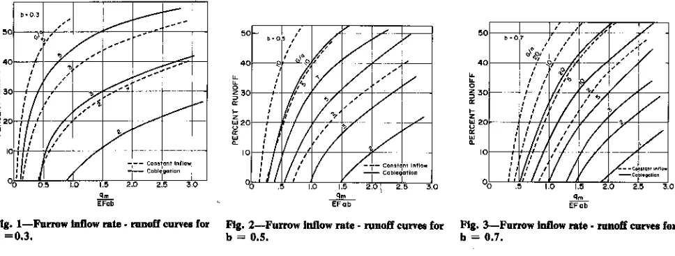
A parameter characterizing the average initial rate of application per unit area is q./(EF), where q. is the initial stream size, E is furrow length and F is furrow spacing. This is divided by the intake rate at one hour, ab, to obtain the dimensionless parameter, q./(EFab). The gross depth of water application, G, is the gross volume applied to a furrow divided by the area, EF. G is divided by the one hour intake depth, a, to obtain the dimensionless parameter, G/a. The percent runoff is third dimensionless parameter.
The assumption is made that the shape of the furrow inflow hydrograph does not change appreciably. The ratio 7q. is slightly affected by the ratio Q/Q,. Values of crcim increase from 0.5 to 0.6 as values of Q/Q, decrease from 0.9 to 0.5. The series of computer runs used to develop the following application intake relationships had values of
Fqm
of about 0.5. Thus, it is assumed that the maximum stream, qm, and gross application, G, which determines the plug speed, completely characterize the furrow inflow distribution. The plug speed, P, is given by the equation,P = K5 Q/(EG) [8 ]
= 60 for Q in L/min, E in m, G in min and P in m /h.
= 8.02 for Q in gal/min, E and G in ft and Pin
-ft/h.
The relationships shown in Figs. 1 to 3 were developed for values of intake parameter b = 0.3, 0.5 and 0.7, respectively. The solid lines were computed from cablegation simulations, with furrow inflow rates starting at q,,, and decreasing to zero. Each line was developed by running a number of simulated irrigations producing a wide range of runoff amounts, and fitting a curve through the calculated points. The dashed curves were computed for constant furrow inflow rate with q. =
ET thus simulating conventional surface irrigation systems. These figures can be used to determine the initial stream size (or constant stream) required for a specified runoff percentage and gross application, given the length of furrow and intake characteristics of the soil. A minimum stream size is needed to produce runoff for a given gross application. The curves represent the range of parameters most likely to occur in practice. The curves will estimate runoff amount or stream size within about 10% accuracy as compared with the computer model. This accuracy is adequate for design purposes since it is difficult to estimate intake rates within 10% and intake rates often vary by a factor of 3 during a single season.
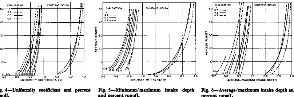
The depth of intake is calculated in the computer model on increments of 10% of the furrow length. The distribution uniformity along a given furrow is characterized by the "Christiansen uniformity coefficient", CU, which is plotted in Fig. 4 as a function of percent runoff and the variables G/a and b. The distribution becomes more uniform as the percent of runoff or gross application increases. Also, the value of b where
K5 K 5
Fig. 1—Furrow inflow rate - runoff curves for b=0.3.
Fig. 2—Furrow inflow rate - runoff curves for b = 0.5.
Pig. 3—Furrow inflow rate - runoff curves for b = 0.7.
CADL E.TION
0 1 — 0.5
CONSTANT INFLOW MI
,., .1 f
::
l I
111
n
iiii ii ii
nn
il
n
,
Nil
mi
ii
,,
m
n
,:,,
nn
r
ill
1j1 I In
62:
08 09 Io 04 09 UNIFORMITY COEFFICIENT,CU
10 .7 0.8 09 10 0.8 09 IA
0.4 08 10 04 06
5191./51.4.% 1HT995 0EPTN
08
04
A/VERAGE/MA315881 INTAKE 08P7H
iliPlum
voill
11
MI
A
...
,, ,
.
.,, .
, ,
,
fti
,li
M /7 I 1
-ir- • Id80 310 51
coNsuudr INFLOW •-.
; 1
0 DS
—.5 •--- I
1
fi
MA
,
i
. An
II F " ii
ril
/ r , !,,
,
,/ 7/
' '
,c .
( 14
50
90
a 20 0
50
40
, 0
a
20
I0
50
0 30
10
Fig. 4—Uniformity coefficient and percent Fig. 5—Minimum/maximum intake depth Fig. 6—Average/maximum intake depth and
runoff. and percent runoff. percent runoff.
has a marked influence on uniformity. Values of CU are given for both the cablegation and constant flow systems. The value of G/a did not influence the CU values for the constant flow case.
The ratio of the minimum intake depth (last 10% of furrow length) to the maximum intake depth (first 10%) is plotted in Fig. 5 as a function of runoff and b. The ratio of the average intake depth (gross depth minus runoff) to the maximum intake depth is similarly plotted in Fig. 6. Several trends are evident from Figs. 4 to 6. For the cablegation system, the uniformity of intake decreases as the value of intake parameter b increases. For the constant inflow system the uniformity is less dependent on b and in fact increases with higher values of b. Thus, it is evident that for soil having high sustained intake rates (b 7 0.5), the constant flow system produces better uniformities, whereas for b < 0.5, the cablegation system produced better uniformities for a given level of runoff. For low runoff amounts the uniformity decreases more rapidly with constant flow than with cablegation. With the average, maximum and minimum intake depths and runoff determined, deep percolation and overall efficiency estimates can be made for given soil water holding capacities and soil depths.
Design Example, field verification and discussion
The use of the figures and equations in designing a cablegation system is illustrated by an example. The data presented by Goel et al. (1982) from an actual field test will be used for comparison. The following parameters are given for this system: S. = 0.0028, C = 150, q =
197 mm, d = 19 mm, Q = 1150 L/min, F = 762 mm, E = 108 m. The intake parameters, a = 19 and b = 0.5 were estimated from the intake rate data given by Goel et al. (1982), using inflow - outflow measurements from eight furrows. The plug speed was P = 6.7 m/h, and the calculated gross application is G = 60 x 11501(108 x 6.7) = 95 ram. The average percent runoff for this field test
was 27%, for all furrows. Entering Fig. 2 with 27% runoff and G/a = 95/19 = 5.0, the value of q.,/(EFab) is found to be 1.3. The predicted maximum size is calculated as 1.3 EFab, or
chr, = 1.3 x 108 m x 0,76 2 m x 19 x 0.5 mm/h
x h160 min = 16.9 L/min
(Note: 1 liter = 1 mm•m2)
The pipe size was 197 min and the outlet size was 19 mm. The pipe flow capacity is Q, = 1462 L/min (equation [1]) and Q/Q, = 0.79. Using equation [2],
= 167 mm, and using equation [4], ch. = 20 L/ min. Using equation [3], X = 84 m and N = 110. Field measurements showed that the actual maximum stream size was about 20 L/min and that about 110 outlets were flowing. A computer simulation of this irrigation using a
= 19.0 and b = 0.5, predicted runoff of 34%.
In this example the stream size predicted by the design curves was about 15% lower than the actual stream size. This is attributed to error in estimation of the intake parameters. If the value of "a" is increased by about 10% to a = 21, G/a = 4.5 and the predicted stream size would increase to q,, = 20 L/min. Thus, the required maximum stream size is sensitive to the intake parameters. As expected, the estimation of intake rates is the weakest link in this design procedure. In a normal design situation the stream size is predicted and then the outlet size is computed. In this case, the predicted stream size was 16.9 L/ min. Equation [5] would predict an outlet size of 16.7 mm for this system.
Figs. 4 to 6 are entered with 27% runoff, b = 0.5 and G/a = 5 resulting in a uniformity coefficient of 0.95, minimum/maximum intake ratio of 0.81, and average/maximum intake depth ratio of 0.92. These parameters were not measured in the field test.
SUMMARY AND CONCLUSIONS
Dimensionless equations were developed to approximate the maximum furrow stream size and the number of flowing outlets for cablegation system with constant outlet size. The maximum outlet pressure head can also be determined directly without computing the entire distribution. If the desired maximum stream size is know, the required outlet size can be determined directly.
Using the two parameter time-based Kostiakov infiltration equation, dimensionless relationships were developed to determine the required maximum stream size the cablegation system given the intake paratmeters, furrow length and spacing, gross water application, percent runoff, and uniformity coefficient. Curves are also presented for the case of constant furrow inflow rate. These relationships comprise a simplified design method for rectangular fields with constant pipe slope. They can be used with the bypass method which maintains uniform applications to furrows while using a constant outlet size. The pipe flow equations can be used alone if the desired stream sizes are known. They can be used in conjunction with the computer model to determine an initial outlet size and reduce the trial and
error process. (continued on page 778)
TRANSACTIONS of the ASAE-1984
Cablegation
(continued from page 772)
The equations can be used to quickly determine the effect of changing the total inflow rate on the outlet head and stream sizes, and uniformity and runoff. Although some outlets to be used with this system are not circular, the system can be designed for circular outlets and then an equivalent noncircular outlet can be selected to give an equivalent area, or head flow relationship.
The cablegation pipe flow equations were developed for specific ranges of the input variables and the user is cautioned to limit use of the equations to those ranges, unless further comparisons are made with the computer model.
The infiltration relationships can be used to design systems for a minimum specified efficiency or uniformity if the intake characteristics are known. Where intake characteristics are expected to vary, a range of required orifice sizes can be determined for systems using adjustable outlets. A maximum furrow length can be determined if a maximum non-erosive stream size is specified. Selection of the adequate levels of uniformity and acceptable runoff amount is left to the designer.
The constant inflow rate curves can be used
independently to determine the required stream size for constant flow surface irrigation systems. They can also be used to make comparisons between cablegation and constant flow systems to determine which system should be used for given soil water intake characteristics. References
1. Goel, M. C. and W. D. Kemper. 1982. Cablegation: III. Field assessment of performance. TRANSACTIONS of the ASAE 25(5): 1304- 1309.
2. Kemper, W. D., W. H. Heinemann, D. C. Kincaid, and R. V. Worstell. 1981. Cablegation: I. Cable controlled plugs in perforated supply pipes for automatic furrow irrigation. TRANSACTIONS of the ASAE 24(6):1526-1532.
3. Kemper, W. D., D. C. Kincaid, R. V. Worstell, W. H. Heinemann, Tom Trout, 3. E. Chapman, F. W. Kemper, and M. Wilson. 1983. Cablegation Type Irrigation Systems: Description, design, installation and performance. To be submitted as a USDA-ARS Western Regional Handbook for publication.
4. Kincaid, D. C. and W. D. Kemper. 1982. Cablegation: II. Simulation and design of the moving-plug gated pipe irrigation system. TRANSACTIONS of the ASAE 25(2):388-395.
5. Kincaid, D. C. and W. D. Kemper. 1984. Cablegation: IV. The bypass method and cutoff outlets to improve water distribution. TRANSACTIONS of the ASAE 27(3):762. 788 (this issue).